Latent Diffusion Models를 사용한 고해상도 이미지 합성

초록

이미지 형성 과정을 denoising autoencoder들의 순차적 적용으로 분해함으로써, diffusion models (DMs)는 이미지 데이터 및 그 너머에서 최첨단 합성 결과를 달성한다. 추가로, 그 정식화는 재훈련 없이 이미지 생성 과정을 제어하는 guiding mechanism을 허용한다. 그러나 이러한 모델들은 일반적으로 pixel space에서 직접 작동하므로, 강력한 DMs의 최적화는 종종 수백 GPU days를 소비하고, inference는 순차적 평가 때문에 비용이 많이 든다. 그 품질과 유연성을 유지하면서 제한된 계산 자원에서 DM 훈련을 가능하게 하기 위해, 우리는 강력한 pretrained autoencoders의 latent space에서 그것들을 적용한다. 이전 연구와 대조적으로, 그러한 표현에서 diffusion models를 훈련하는 것은 복잡도 감소와 세부 보존 사이의 거의 최적 지점에 처음으로 도달하게 하며, 시각적 충실도를 크게 향상시킨다. 모델 아키텍처에 cross-attention layers를 도입함으로써, 우리는 diffusion models를 텍스트나 bounding boxes와 같은 일반 conditioning inputs를 위한 강력하고 유연한 생성기로 바꾸며, high-resolution synthesis는 convolutional 방식으로 가능해진다. 우리의 latent diffusion models (LDMs)는 image inpainting과 class-conditional image synthesis에서 새로운 state-of-the-art 점수를 달성하고, text-to-image synthesis, unconditional image generation 및 super-resolution을 포함한 다양한 작업에서 매우 경쟁력 있는 성능을 달성하면서, pixel-based DMs에 비해 계산 요구량을 크게 줄인다.

1 서론

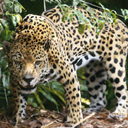
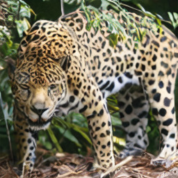
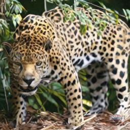
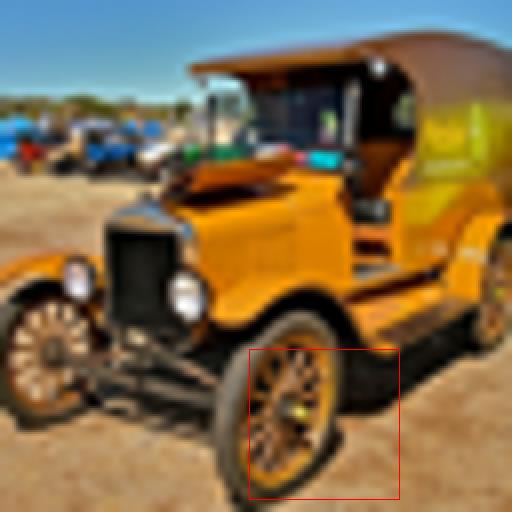
입력 ours ($f=4$) PSNR:$27.4$R-FID:$0.58$ DALL-E ($f=8$) PSNR:$22.8$R-FID:$32.01$ VQGAN ($f=16$) PSNR:$19.9$R-FID:$4.98$

Figure 1: 덜 공격적인 downsampling으로 달성 가능한 품질의 상한을 높이기. diffusion models는 spatial data에 대한 뛰어난 inductive biases를 제공하므로, 우리는 latent space의 관련 generative models에서처럼 무거운 spatial downsampling이 필요하지 않지만, 적절한 autoencoding models를 통해 데이터의 dimensionality를 여전히 크게 줄일 수 있다. Sec. 참조3. 이미지들은 DIV2K에서 왔다[1]validation set이며, 다음에서 평가됨${512}^2$px. 우리는 spatial downsampling factor를 다음으로 표시한다$f$. Reconstruction FIDs[29]및 PSNR은 ImageNet-val에서 계산된다.[12]; Tab.도 참조8.

이미지 합성은 가장 눈부신 최근 발전을 보인 컴퓨터 비전 분야 중 하나이지만, 동시에 가장 큰 계산 요구를 가진 분야들 중 하나이기도 하다. 특히 복잡한 자연 장면의 고해상도 합성은 현재 autoregressive (AR) transformers에서 잠재적으로 수십억 개의 parameters를 포함하는 likelihood-based models의 scaling up이 지배하고 있다[66, 67]. 대조적으로, GANs의 유망한 결과는[27, 3, 40]그 adversarial learning procedure가 복잡한 multi-modal distributions의 modeling으로 쉽게 scale하지 않기 때문에, 비교적 제한된 variability를 가진 데이터에 대부분 국한되는 것으로 드러났다. 최근 diffusion models[82], denoising autoencoders의 hierarchy로 구축되는, 는 image synthesis에서 인상적인 결과를 달성함을 보였다[30, 85]및 그 너머에서[45, 7, 48, 57], 그리고 class-conditional image synthesis에서 state-of-the-art를 정의한다[15, 31]및 super-resolution에서[72]. 더욱이, unconditional DMs조차 inpainting과 colorization 같은 작업에 쉽게 적용될 수 있다[85]또는 stroke-based synthesis[53], 다른 유형의 generative models와 대조적으로[46, 69, 19]. likelihood-based models이기 때문에, 이들은 GANs와 같은 mode-collapse 및 training instabilities를 보이지 않으며, parameter sharing을 크게 활용함으로써 AR models에서처럼 수십억 개의 parameters를 포함하지 않고도 자연 이미지의 매우 복잡한 distributions를 모델링할 수 있다[67].

고해상도 이미지 합성의 민주화

DMs는 likelihood-based models의 부류에 속하며, 그 mode-covering behavior는 데이터의 지각할 수 없는 세부사항을 모델링하는 데 과도한 양의 capacity(따라서 compute resources)를 쓰기 쉽게 만든다[16, 73]. reweighted variational objective가[30]초기 denoising steps를 undersampling함으로써 이를 해결하는 것을 목표로 하지만, DMs는 여전히 계산적으로 요구가 크다. 그러한 모델을 훈련하고 평가하려면 RGB 이미지의 고차원 공간에서 반복적인 function evaluations(및 gradient computations)이 필요하기 때문이다. 예로서, 가장 강력한 DMs를 훈련하는 것은 종종 수백 GPU days가 걸린다 (e.g.150 - 1000 V100 days in[15]) 그리고 input space의 noisy version에 대한 반복 평가도 inference를 비싸게 만들어, 50k samples를 생성하는 데 약 5 days가 걸린다[15]단일 A100 GPU에서. 이는 research community와 일반 users에게 두 가지 결과를 낳는다: 첫째, 그러한 모델을 훈련하려면 해당 분야의 소수에게만 उपलब्ध한 막대한 계산 자원이 필요하며, 거대한 carbon footprint를 남긴다[65, 86]. 둘째, 이미 훈련된 모델을 평가하는 것도 시간과 메모리 면에서 비싸다. 동일한 model architecture가 많은 수의 steps 동안 순차적으로 실행되어야 하기 때문이다 (e.g.25 - 1000 steps in[15]).

이 강력한 model class의 접근성을 높이는 동시에 그 상당한 자원 소비를 줄이기 위해, training과 sampling 모두에 대한 computational complexity를 줄이는 방법이 필요하다. 따라서 성능을 저해하지 않고 DMs의 계산 요구를 줄이는 것은 그 접근성을 향상시키는 핵심이다.

Latent Space로의 출발

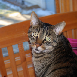
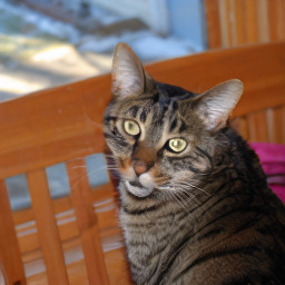
우리의 접근은 pixel space에서 이미 훈련된 diffusion models의 분석으로 시작한다: Fig.2는 훈련된 모델의 rate-distortion trade-off를 보여준다. 어떤 likelihood-based model과 마찬가지로, learning은 대략 두 단계로 나눌 수 있다: 첫 번째는perceptual compression단계로, high-frequency details를 제거하지만 여전히 semantic variation은 거의 학습하지 않는다. 두 번째 단계에서 실제 generative model은 데이터의 semantic and conceptual composition을 학습한다 (semantic compression). 따라서 우리는 먼저 찾는 것을 목표로 한다지각적으로 동등하지만 계산적으로 더 적합한 공간, 그 안에서 우리는 high-resolution image synthesis를 위한 diffusion models를 훈련할 것이다.

일반적인 관행을 따라[96, 67, 23, 11, 66], 우리는 training을 두 개의 구별된 phases로 분리한다: 먼저, data space와 지각적으로 동등한 lower-dimensional(따라서 efficient) representational space를 제공하는 autoencoder를 훈련한다. 중요하게도, 이전 연구와 대조적으로[23, 66], 우리는 과도한 spatial compression에 의존할 필요가 없다. 우리는 학습된 latent space에서 DMs를 훈련하며, 이는 spatial dimensionality와 관련하여 더 나은 scaling properties를 보이기 때문이다. 감소된 complexity는 또한 단일 network pass로 latent space에서 효율적인 image generation을 제공한다. 우리는 결과 model class를 다음으로 부른다Latent Diffusion Models(LDMs).

이 접근의 주목할 만한 장점은 universal autoencoding stage를 한 번만 훈련하면 되며, 따라서 이를 여러 DM trainings에 재사용하거나 가능하게는 완전히 다른 tasks를 탐색하는 데 재사용할 수 있다는 점이다[81]. 이는 다양한 image-to-image 및 text-to-image tasks를 위한 많은 수의 diffusion models를 효율적으로 탐색하게 한다. 후자를 위해, 우리는 transformers를 DM의 UNet backbone에 연결하는 architecture를 설계한다[71]그리고 임의 유형의 token-based conditioning mechanisms를 가능하게 한다. Sec. 참조3.3.

Figure 2: perceptual 및 semantic compression 설명: 디지털 이미지의 대부분의 bits는 지각할 수 없는 세부사항에 해당한다. DMs는 responsible loss term을 최소화하여 이 의미론적으로 무의미한 정보를 억제할 수 있게 하지만, gradients(훈련 중)와 neural network backbone(training 및 inference)은 여전히 모든 pixels에서 평가되어야 하며, 이는 불필요한 계산과 불필요하게 비싼 optimization 및 inference로 이어진다.
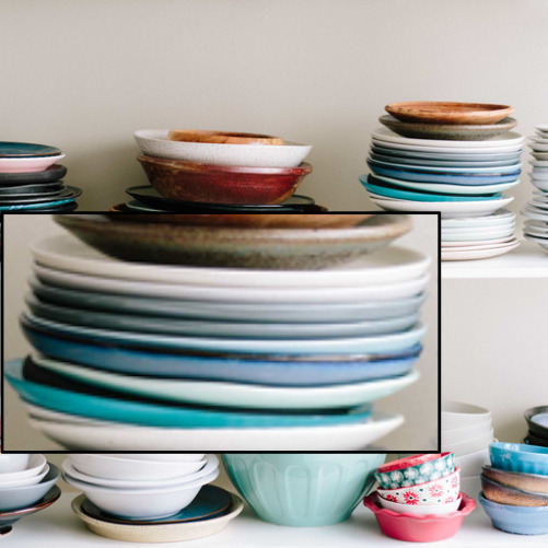
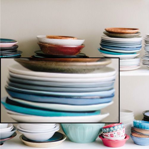
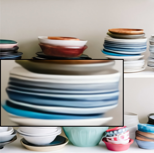
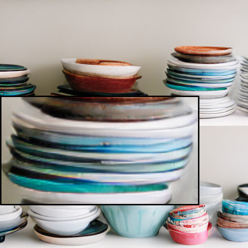
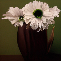
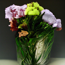
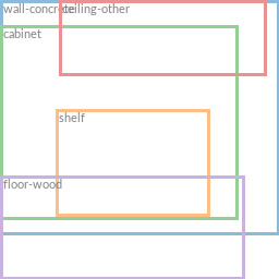
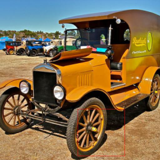
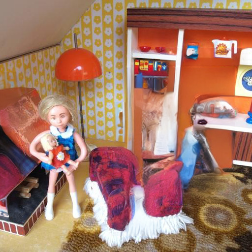
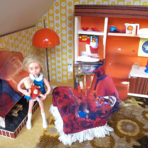
우리는 제안한다latent diffusion models (LDMs)효과적인 generative model 및 지각할 수 없는 세부사항만 제거하는 별도의 mild compression stage로서. 데이터와 이미지는 다음에서 왔다[30].

요컨대, 우리의 작업은 다음의기여:

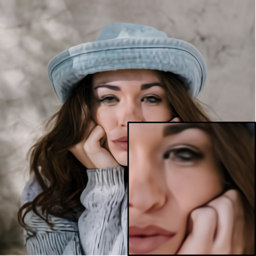
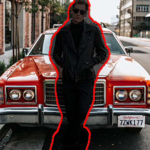
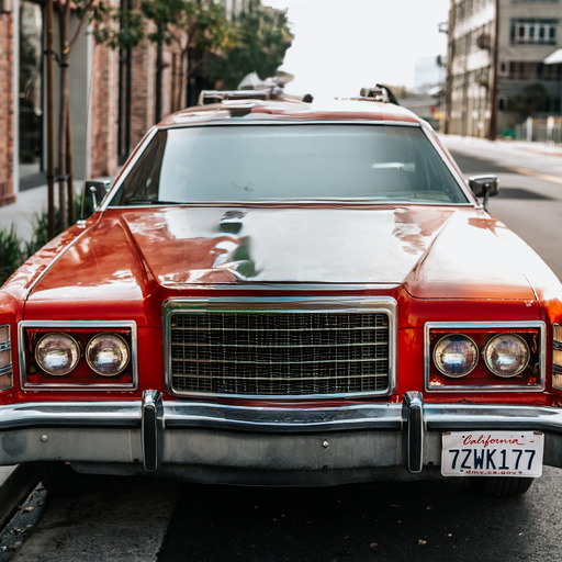
(i) 순수하게 transformer-based approaches와 대조적으로[23, 66], 우리의 방법은 더 높은 dimensional data로 더 우아하게 scale하며 따라서 (a) 이전 연구보다 더 충실하고 상세한 reconstructions를 제공하는 compression level에서 작동할 수 있고(Fig. 참조1) 그리고 (b) megapixel images의 high-resolution synthesis에 효율적으로 적용될 수 있다.

(ii) 우리는 computational costs를 크게 낮추면서 여러 tasks(unconditional image synthesis, inpainting, stochastic super-resolution)와 datasets에서 경쟁력 있는 성능을 달성한다. pixel-based diffusion approaches와 비교하여, 우리는 inference costs도 크게 줄인다.

(iii) 우리는 이전 연구와 대조적으로 보여준다[93]encoder/decoder architecture와 score-based prior를 동시에 학습하는, 우리의 접근은 reconstruction과 generative abilities의 섬세한 weighting을 필요로 하지 않는다. 이는 극히 충실한 reconstructions를 보장하며 latent space의 regularization을 매우 적게 요구한다.

(iv) 우리는 super-resolution, inpainting 및 semantic synthesis와 같이 densely conditioned tasks의 경우, 우리의 모델이 convolutional fashion으로 적용될 수 있고 다음 크기의 크고 일관된 images를 render할 수 있음을 발견했다$\sim {1024}^2$px.

(v) 더욱이, 우리는 cross-attention에 기반한 general-purpose conditioning mechanism을 설계하여 multi-modal training을 가능하게 한다. 우리는 이를 사용해 class-conditional, text-to-image 및 layout-to-image models를 훈련한다.

(vi) 마지막으로, 우리는 pretrained latent diffusion 및 autoencoding models를 다음에 공개한다https://github.com/CompVis/latent-diffusion이는 DMs의 training 외에도 다양한 tasks에 재사용될 수 있다[81].

2 관련 연구

이미지 합성을 위한 Generative Models이미지의 고차원적 성격은 generative modeling에 뚜렷한 도전 과제를 제시한다. Generative Adversarial Networks (GAN)[27]좋은 perceptual quality를 가진 high resolution images의 효율적인 sampling을 가능하게 한다[3, 42], 그러나 optimize하기 어렵다[54, 2, 28]그리고 전체 data distribution을 포착하는 데 어려움을 겪는다[55]. 대조적으로, likelihood-based methods는 good density estimation을 강조하며 이는 optimization을 더 well-behaved하게 만든다. Variational autoencoders (VAE)[46]및 flow-based models[18, 19]high resolution images의 효율적인 synthesis를 가능하게 한다[9, 92, 44], 그러나 sample quality는 GANs와 동등하지 않다. autoregressive models (ARM)가[95, 94, 6, 10]density estimation에서 강력한 성능을 달성하지만, computationally demanding architectures[97]및 sequential sampling process는 그것들을 low resolution images로 제한한다. 이미지의 pixel based representations는 거의 지각할 수 없는 high-frequency details를 포함하기 때문에[16, 73], maximum-likelihood training은 그것들을 모델링하는 데 불균형적으로 많은 capacity를 사용하여 긴 training times를 초래한다. 더 높은 resolutions로 scale하기 위해, 여러 two-stage approaches는[101, 67, 23, 103]raw pixels 대신 compressed latent image space를 모델링하기 위해 ARMs를 사용한다.

최근,Diffusion Probabilistic Models(DM)[82], 는 density estimation에서 state-of-the-art results를 달성했다[45]뿐만 아니라 sample quality에서도[15]. 이러한 모델들의 generative power는 그 underlying neural backbone이 UNet으로 구현될 때 image-like data의 inductive biases에 자연스럽게 맞는 데서 비롯된다[71, 30, 85, 15]. 최고의 synthesis quality는 보통 reweighted objective가[30]training에 사용될 때 달성된다. 이 경우 DM은 lossy compressor에 해당하며 image quality를 compression capabilities와 trade할 수 있게 한다. 그러나 pixel space에서 이러한 모델들을 평가하고 optimize하는 것은 낮은 inference speed와 매우 높은 training costs라는 단점이 있다. 전자는 advanced sampling strategies에 의해 부분적으로 해결될 수 있지만[84, 75, 47]및 hierarchical approaches[31, 93], high-resolution image data에서의 training은 항상 expensive gradients를 계산해야 한다. 우리는 제안한 다음으로 두 단점을 모두 해결한다LDMs, 이는 더 낮은 dimensionality의 compressed latent space에서 작동한다. 이는 training을 computationally cheaper하게 만들고 synthesis quality의 거의 감소 없이 inference를 가속한다(Fig. 참조1).

Two-Stage Image Synthesis개별 generative approaches의 단점을 완화하기 위해, 많은 연구가[11, 70, 23, 103, 101, 67]two stage approach를 통해 서로 다른 methods의 장점을 더 효율적이고 성능 좋은 models로 결합하는 데 들어갔다. VQ-VAEs는[101, 67]discretized latent space 위의 expressive prior를 학습하기 위해 autoregressive models를 사용한다.[66]discretized image 및 text representations에 대한 joint distributation을 학습함으로써 이 접근을 text-to-image generation으로 확장한다. 더 일반적으로,[70]conditionally invertible networks를 사용하여 다양한 domains의 latent spaces 사이의 generic transfer를 제공한다. VQ-VAEs와 달리, VQGANs는[23, 103]autoregressive transformers를 더 큰 images로 scale하기 위해 adversarial 및 perceptual objective를 가진 first stage를 사용한다. 그러나 feasible ARM training에 필요한 높은 compression rates는 수십억 개의 trainable parameters를 도입하며[66, 23], 그러한 approaches의 전체 performance를 제한하고, 적은 compression은 높은 computational cost라는 대가를 치른다[66, 23]. 우리의 작업은 그러한 trade-offs를 방지한다. 우리가 제안한LDMs는 convolutional backbone 덕분에 더 높은 dimensional latent spaces로 더 완만하게 scale하기 때문이다. 따라서 우리는 고충실도 reconstructions를 보장하면서 generative diffusion model에 너무 많은 perceptual compression을 남기지 않고 강력한 first stage 학습 사이를 최적으로 중재하는 compression level을 자유롭게 선택할 수 있다(Fig. 참조1).

공동으로[93]또는 별도로[80]score-based prior와 함께 encoding/decoding model을 학습하는 접근들이 존재하지만, 전자는 여전히 reconstruction과 generative capabilities 사이의 어려운 weighting을 요구한다[11]그리고 우리의 접근보다 성능이 낮으며(Sec.4), 후자는 human faces와 같은 고도로 structured images에 초점을 맞춘다.

3 방법

고해상도 이미지 합성을 향한 diffusion models training의 계산 요구를 낮추기 위해, 우리는 diffusion models가 해당 loss terms를 undersampling함으로써 perceptually irrelevant details를 무시할 수 있게 하지만[30], 여전히 pixel space에서 costly function evaluations를 요구하며, 이는 computation time과 energy resources에서 막대한 요구를 초래한다는 것을 관찰한다.

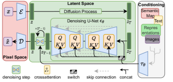
우리는 compressive learning phase와 generative learning phase의 명시적 분리를 도입함으로써 이 단점을 우회할 것을 제안한다(Fig. 참조2). 이를 달성하기 위해, 우리는 image space와 지각적으로 동등하지만 computational complexity를 크게 줄인 공간을 학습하는 autoencoding model을 활용한다.

그러한 접근은 여러 장점을 제공한다: (i) 고차원 image space를 떠남으로써, sampling이 low-dimensional space에서 수행되기 때문에 계산적으로 훨씬 더 효율적인 DMs를 얻는다. (ii) 우리는 DMs가 그 UNet architecture에서 물려받은 inductive bias를 활용한다[71], 이는 spatial structure를 가진 데이터에 특히 효과적이게 하며 따라서 이전 approaches가 요구한 공격적이고 품질을 낮추는 compression levels의 필요를 완화한다[23, 66]. (iii) 마지막으로, 우리는 latent space가 여러 generative models를 훈련하는 데 사용될 수 있고 single-image CLIP-guided synthesis와 같은 다른 downstream applications에도 활용될 수 있는 general-purpose compression models를 얻는다[25].

3.1 Perceptual Image Compression

우리의 perceptual compression model은 이전 연구에 기반한다[23]그리고 perceptual loss의 조합으로 훈련된 autoencoder로 구성된다[106]및 patch-based[33]adversarial objective[20, 23, 103]. 이는 local realism을 강제함으로써 reconstructions가 image manifold에 국한되도록 보장하고, 다음과 같은 pixel-space losses에만 의존함으로써 도입되는 bluriness를 피한다$L_2$또는$L_1$objectives.

더 정확히는, 이미지가 주어졌을 때$x\in {ℝ}^{H\times W\times 3}$RGB space에서, encoder$ℰ$는 인코딩한다$x$latent representation으로$z=ℰ\left(x\right)$, 그리고 decoder$𝒟$는 latent로부터 이미지를 reconstruct하여 다음을 제공한다$\tilde{x}=𝒟\left(z\right)=𝒟\left(ℰ\left(x\right)\right)$, 여기서$z\in {ℝ}^{h\times w\times c}$. 중요하게도, encoder는downsamples이미지를 factor만큼$f=H/h=W/w$, 그리고 우리는 서로 다른 downsampling factors를 조사한다$f=2^m$, with$m\in \mathbb{N}$.

임의로 높은 variance의 latent spaces를 피하기 위해, 우리는 두 가지 다른 종류의 regularizations를 실험한다. 첫 번째 변형,KL-reg., 는 VAE와 유사하게 학습된 latent에 대해 standard normal을 향한 약한 KL-penalty를 부과한다[46, 69], whereasVQ-reg.는 vector quantization layer를 사용한다[96]decoder 내부에서. 이 모델은 VQGAN으로 해석될 수 있다[23]하지만 quantization layer가 decoder에 흡수된 것이다. 우리의 후속 DM은 학습된 latent space의 two-dimensional structure와 함께 작동하도록 설계되었기 때문에$z=ℰ\left(x\right)$, 우리는 비교적 mild compression rates를 사용하고 매우 좋은 reconstructions를 달성할 수 있다. 이는 이전 연구들과 대조적이다[23, 66], 이들은 학습된 space의 임의의 1D ordering에 의존했다$z$그 distribution을 autoregressively 모델링하고 따라서 다음의 inherent structure의 많은 부분을 무시하기 위해$z$. 따라서, 우리의 compression model은 다음의 details를 보존한다$x$더 잘(Tab. 참조8). 전체 objective와 training details는 supplement에서 찾을 수 있다.

3.2 Latent Diffusion Models

Diffusion Models [82]는 data distribution을 학습하도록 설계된 probabilistic models이다$p\left(x\right)$normally distributed variable을 점진적으로 denoising함으로써, 이는 length가 다음인 고정 Markov Chain의 reverse process를 학습하는 것에 해당한다$T$. image synthesis의 경우, 가장 성공적인 models는[30, 15, 72]다음에 대한 variational lower bound의 reweighted variant에 의존한다$p\left(x\right)$, 이는 denoising score-matching을 반영한다[85]. 이러한 models는 동일하게 weighted된 denoising autoencoders의 sequence로 해석될 수 있다${ϵ}_{\theta }(x_t,t);t=1\dots T$, 이들은 input의 denoised variant를 예측하도록 훈련된다$x_t$, 여기서$x_t$는 input의 noisy version이다$x$. 해당 objective는 다음으로 단순화될 수 있다(Sec.B)

$L_{DM}={𝔼}_{x,ϵ\sim 𝒩(0,1),t}\left[{\Vert ϵ-{ϵ}_{\theta }(x_t,t)\Vert }_2^2\right],$ (1)

with$t$에서 uniform하게 sampled된$\{1,\dots ,T\}$.

Latent Representations의 Generative Modeling다음으로 구성된 우리의 훈련된 perceptual compression models로$ℰ$그리고$𝒟$, 우리는 이제 high-frequency, imperceptible details가 abstracted away된 효율적인 low-dimensional latent space에 접근할 수 있다. 고차원 pixel space와 비교하여, 이 space는 likelihood-based generative models에 더 적합하다. 이제 이들은 (i) 데이터의 중요하고 semantic한 bits에 집중할 수 있고 (ii) 더 낮은 dimensional, computationally much more efficient space에서 훈련할 수 있기 때문이다.

고도로 compressed, discrete latent space에서 autoregressive, attention-based transformer models에 의존한 이전 연구와 달리[66, 23, 103], 우리는 우리 모델이 제공하는 image-specific inductive biases를 활용할 수 있다. 여기에는 underlying UNet을 주로 2D convolutional layers로 구축하는 능력, 그리고 reweighted bound를 사용하여 perceptually most relevant bits에 objective를 더 집중하는 것이 포함되며, 이제 이는 다음과 같이 읽힌다

Figure 3: 우리는 LDMs를 concatenation을 통해 또는 더 일반적인 cross-attention mechanism으로 condition한다. Sec. 참조3.3

$L_{LDM}:={𝔼}_{ℰ\left(x\right),ϵ\sim 𝒩(0,1),t}\left[{\Vert ϵ-{ϵ}_{\theta }(z_t,t)\Vert }_2^2\right].$ (2)

neural backbone${ϵ}_{\theta }(\circ ,t)$우리 모델의 는 time-conditional UNet으로 구현된다[71]. forward process가 고정되어 있으므로,$z_t$는 효율적으로 얻을 수 있다, 다음으로부터$ℰ$training 중에, 그리고 다음으로부터의 samples$p(z$)는 단 한 번의 통과로 이미지 공간으로 디코딩될 수 있다$𝒟$.

CelebAHQ			FFHQ			LSUN-Churches			LSUN-Beds			ImageNet

Figure 4: 다음으로부터의 샘플LDMsCelebAHQ에서 학습된[39], FFHQ[41], LSUN-Churches[102], LSUN-Bedrooms[102]및 class-conditional ImageNet[12], 각각의 해상도는$256\times 256$. 확대해서 볼 때 가장 좋다. 더 많은 샘플은cf.부록을 보라.

3.3 컨디셔닝 메커니즘

다른 유형의 생성 모델들과 유사하게[56, 83], diffusion model은 원칙적으로 다음 형태의 조건부 분포를 모델링할 수 있다$p\left(z|y\right)$. 이는 조건부 denoising autoencoder로 구현될 수 있다${ϵ}_{\theta }(z_t,t,y)$그리고 입력을 통해 합성 과정을 제어하는 길을 연다$y$텍스트와 같은[68], semantic map[61, 33]또는 다른 image-to-image translation 작업[34].

그러나 이미지 합성의 맥락에서, DM의 생성 능력을 class-label을 넘어서는 다른 유형의 conditioning과 결합하는 것은[15]또는 입력 이미지의 흐릿한 변형[72]지금까지 충분히 탐구되지 않은 연구 영역이다.

우리는 그 기반 UNet backbone에 cross-attention mechanism을 추가함으로써 DM을 더 유연한 조건부 이미지 생성기로 바꾼다[97], 이는 다양한 입력 modality의 attention 기반 모델을 학습하는 데 효과적이다[36, 35]. 전처리하기 위해$y$다양한 modality(예: language prompt)로부터 우리는 domain specific encoder를 도입한다${\tau }_{\theta }$이는 투영한다$y$중간 표현으로${\tau }_{\theta }\left(y\right)\in {ℝ}^{M\times d_{\tau }}$, 이는 그런 다음 구현하는 cross-attention layer를 통해 UNet의 중간 layer들에 매핑된다$\text{Attention}(Q,K,V)=\text{softmax}\left(\frac{Q{K}^T}{\sqrt{d}}\right)\cdot V$, 여기서

$Q=W_Q^{\left(i\right)}\cdot {\phi }_i\left(z_t\right),K=W_K^{\left(i\right)}\cdot {\tau }_{\theta }\left(y\right),V=W_V^{\left(i\right)}\cdot {\tau }_{\theta }\left(y\right).$

여기서,${\phi }_i\left(z_t\right)\in {ℝ}^{N\times d_{ϵ}^i}$구현하는 UNet의 (평탄화된) 중간 표현을 나타낸다${ϵ}_{\theta }$그리고$W_V^{\left(i\right)}\in {ℝ}^{d\times d_{ϵ}^i}$, $W_Q^{\left(i\right)}\in {ℝ}^{d\times d_{\tau }}$ & $W_K^{\left(i\right)}\in {ℝ}^{d\times d_{\tau }}$학습 가능한 projection matrix들이다[97, 36]. 시각적 묘사는 Fig.를 보라3.

이미지-conditioning 쌍을 기반으로, 우리는 그런 다음 다음을 통해 conditional LDM을 학습한다

$L_{LDM}:={𝔼}_{ℰ\left(x\right),y,ϵ\sim 𝒩(0,1),t}\left[{\Vert ϵ-{ϵ}_{\theta }(z_t,t,{\tau }_{\theta }\left(y\right))\Vert }_2^2\right],$ (3)

여기서 둘 다${\tau }_{\theta }$그리고${ϵ}_{\theta }$Eq.를 통해 공동으로 최적화된다3. 이 conditioning mechanism은 유연한데, 이는${\tau }_{\theta }$domain-specific expert로 매개변수화될 수 있기 때문이다,e.g.(unmasked) transformer[97]다음일 때$y$텍스트 prompt이다(Sec. 참조4.3.1)

4 실험

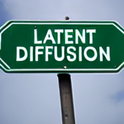
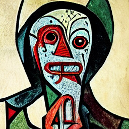
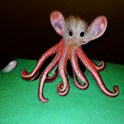
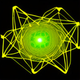
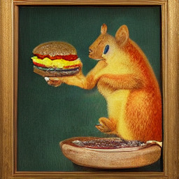
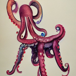
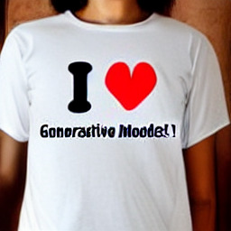
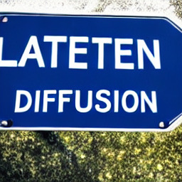
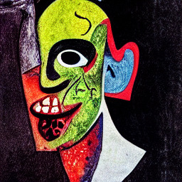
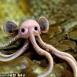
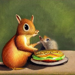
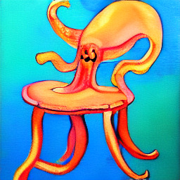
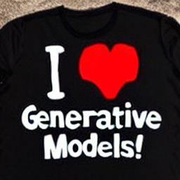
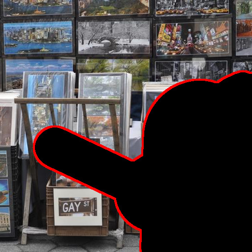
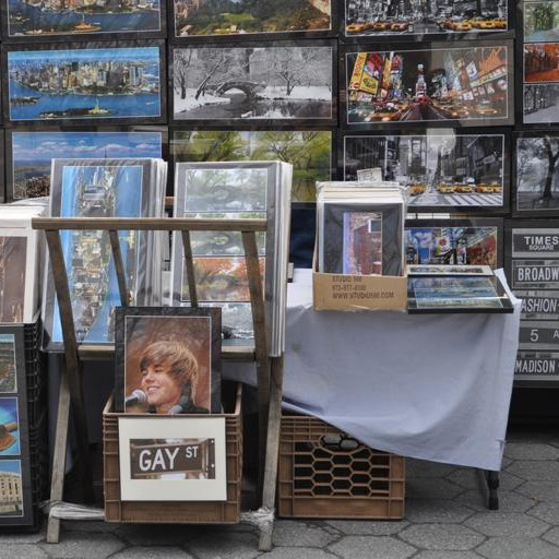
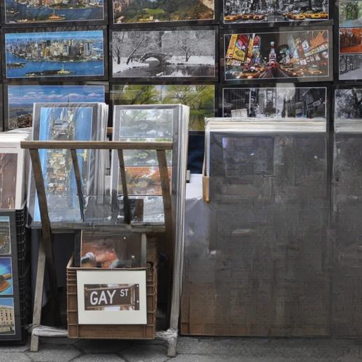
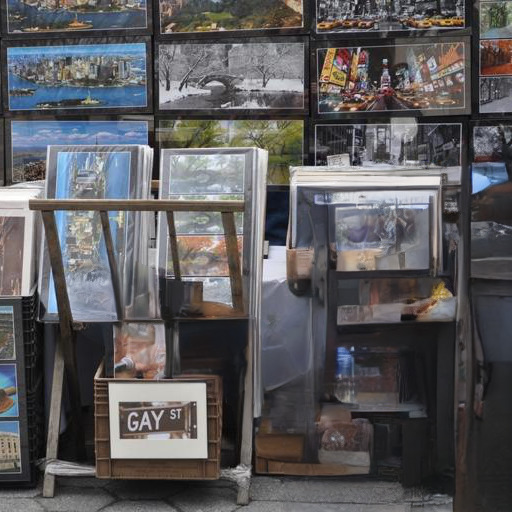
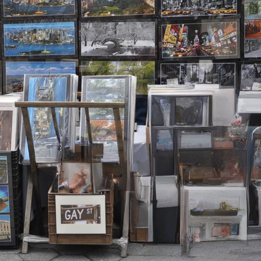
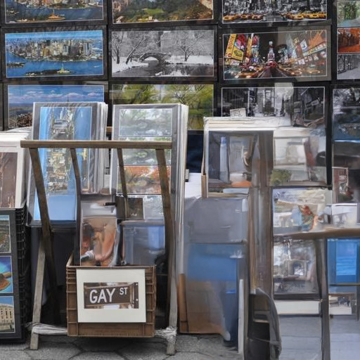
LAION에서의 Text-to-Image Synthesis. 1.45B Model.
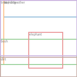
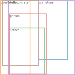
’다음이라고 적힌 거리 표지판 “Latent Diffusion” ’	’Picasso의 스타일의 좀비’	’반은 mouse이고 반은 octopus인 동물의 이미지’	’약간 의식이 있는 neural network의 illustration’	’burger를 먹고 있는 squirrel의 그림’	’octopus처럼 보이는 chair의 watercolor painting’	’다음 문구가 적힌 shirt: “I love generative models!” ’

Figure 5: text-to-image synthesis를 위한 우리 모델에서 사용자 정의 text prompt에 대한 샘플,LDM-8 (KL), 이는 LAION에서 학습되었다[78]database. 샘플은 200 DDIM step과 함께 생성되었고$\eta =1.0$. 우리는 unconditional guidance를 사용한다[32]다음과 함께$s=10.0$.

Figure 6: class-conditional 학습 분석LDMs서로 다른 downsampling factor를 가진$f$ImageNet dataset에서 2M train step 동안. Pixel-basedLDM-1은 더 큰 downsampling factor를 가진 모델들에 비해 상당히 더 큰 학습 시간을 요구한다 (LDM-$\{$4-16$\}$). 다음과 같은 너무 많은 perceptual compression은LDM-32전체 sample quality를 제한한다. 모든 모델은 동일한 computational budget으로 단일 NVIDIA A100에서 학습된다. 결과는 100 DDIM step으로 얻었다[84]그리고$\kappa =0$.

Figure 7: 비교LDMsCelebA-HQ(왼쪽)와 ImageNet(오른쪽) dataset에서 다양한 compression을 가진. 서로 다른 marker는 나타낸다$\{10,20,50,100,200\}$DDIM을 사용하는 sampling step을, 각 선을 따라 오른쪽에서 왼쪽으로. 점선은 200 step에 대한 FID score를 보여주며, 다음의 강한 성능을 나타낸다LDM-$\{$4-8$\}$. FID score는 5000개 sample에서 평가되었다. 모든 모델은 A100에서 500k(CelebA) / 2M(ImageNet) step 동안 학습되었다.

LDMs는 다양한 이미지 modality의 유연하고 계산적으로 다루기 쉬운 diffusion 기반 이미지 합성 수단을 제공하며, 이를 다음에서 경험적으로 보인다. 그러나 먼저, 우리는 학습과 추론 모두에서 pixel-based diffusion model과 비교하여 우리 모델의 이득을 분석한다. 흥미롭게도, 우리는 다음을 발견한다LDMs에서 학습된VQ-regularized latent space는 때때로 더 나은 sample quality를 달성한다, 비록 다음의 reconstruction capability가VQ-regularized first stage model은 연속적인 대응 모델보다 약간 뒤처지지만,cf.Tab.8. first stage regularization scheme이 다음에 미치는 효과에 대한 시각적 비교는LDM학습과 해상도에 대한 이들의 일반화 능력$>{256}^2$Appendix에서 찾을 수 있다D.1. 다음에서E.2우리는 이 절에 제시된 모든 결과에 대한 architecture, implementation, training 및 evaluation의 세부사항을 나열한다.

4.1 Perceptual Compression Tradeoff에 관하여

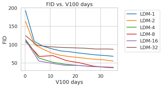
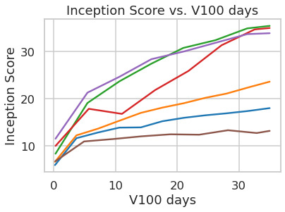
이 절은 서로 다른 downsampling factor를 가진 우리 LDM의 동작을 분석한다$f\in \{1,2,4,8,16,32\}$(다음으로 축약됨LDM-$f$, 여기서LDM-1은 pixel-based DM에 해당한다). 비교 가능한 test-field를 얻기 위해, 우리는 이 절의 모든 실험에서 계산 자원을 단일 NVIDIA A100으로 고정하고, 모든 모델을 동일한 step 수와 동일한 parameter 수로 학습한다.

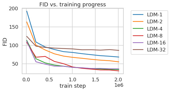
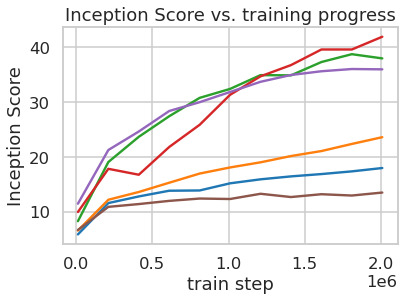
Tab.8는 다음을 위해 사용된 first stage model의 hyperparameter와 reconstruction performance를 보여준다LDMs이 절에서 비교된. Fig.6는 ImageNet에서 class-conditional model의 2M step 동안 training progress의 함수로 sample quality를 보여준다[12]dataset. 우리는 다음을 본다, i) 다음에 대한 작은 downsampling factor는LDM-$\{$1,2$\}$느린 training progress를 초래하는 반면, ii) 지나치게 큰 값의$f$비교적 적은 training step 후에 fidelity가 정체되게 한다. 위의 분석(Fig.1그리고2)을 다시 살펴보면, 우리는 이를 i) perceptual compression의 대부분을 diffusion model에 남겨두는 것과 ii) 너무 강한 first stage compression이 정보 손실을 초래하여 달성 가능한 quality를 제한하는 것에 기인한다고 본다.LDM-$\{$4-16$\}$는 효율성과 지각적으로 충실한 결과 사이의 좋은 균형을 이루며, 이는 유의미한 FID로 나타난다[29]pixel-based diffusion (LDM-1)와LDM-8사이의 2M training step 후 gap 38.

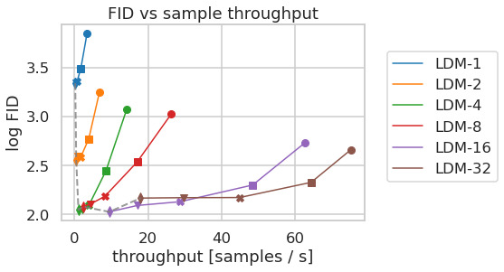
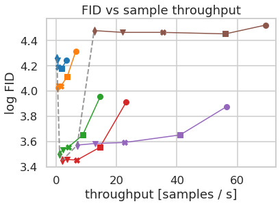
Fig.에서7, 우리는 CelebA-HQ에서 학습된 모델을 비교한다[39]그리고 ImageNet을 DDIM sampler를 사용한 서로 다른 수의 denoising step에 대한 sampling speed 측면에서[84]그리고 이를 FID-score에 대해 plot한다[29]. LDM-$\{$4-8$\}$는 perceptual compression과 conceptual compression의 부적절한 비율을 가진 모델보다 우수하다. 특히 pixel-based와 비교하여LDM-1, 이들은 동시에 sample throughput을 크게 증가시키면서 훨씬 더 낮은 FID score를 달성한다. ImageNet과 같은 복잡한 dataset은 quality 저하를 피하기 위해 감소된 compression rate를 요구한다. 요약하면,LDM-4그리고-8고품질 합성 결과를 달성하기 위한 최상의 조건을 제공한다.

CelebA-HQ$256\times 256$ FFHQ$256\times 256$ 방법 FID$\downarrow$ Prec.$\uparrow$ Recall$\uparrow$ 방법 FID$\downarrow$ Prec.$\uparrow$ Recall$\uparrow$ DC-VAE[63] 15.8 - - ImageBART[21] 9.57 - - VQGAN+T.[23] (k=400) 10.2 - - U-Net GAN (+aug)[77] 10.9 (7.6) - - PGGAN[39] 8.0 - - UDM[43] 5.54 - - LSGM[93] 7.22 - - StyleGAN[41] 4.16 0.71 0.46 UDM[43] 7.16 - - ProjectedGAN[76] 3.08 0.65 0.46 LDM-4(ours, 500-s^†) 5.11 0.72 0.49 LDM-4(ours, 200-s) 4.98 0.73 0.50

LSUN-Churches$256\times 256$ LSUN-Bedrooms$256\times 256$ 방법 FID$\downarrow$ Prec.$\uparrow$ Recall$\uparrow$ 방법 FID$\downarrow$ Prec.$\uparrow$ Recall$\uparrow$ DDPM[30] 7.89 - - ImageBART[21] 5.51 - - ImageBART[21] 7.32 - - DDPM[30] 4.9 - - PGGAN[39] 6.42 - - UDM[43] 4.57 - - StyleGAN[41] 4.21 - - StyleGAN[41] 2.35 0.59 0.48 StyleGAN2[42] 3.86 - - ADM[15] 1.90 0.66 0.51 ProjectedGAN[76] 1.59 0.61 0.44 ProjectedGAN[76] 1.52 0.61 0.34 LDM-8^∗(ours, 200-s) 4.02 0.64 0.52 LDM-4(ours, 200-s) 2.95 0.66 0.48

Table 1: 무조건부 이미지 합성을 위한 evaluation metric. CelebA-HQ 결과는 다음에서 재현됨[63, 100, 43], FFHQ는 다음에서[42, 43]. ^†: $N$-s는 다음을 가리킨다$N$DDIM을 사용한 샘플링 단계[84]샘플러.^∗: 다음에서 학습됨KL-정규화된 latent space. 추가 결과는 supplementary에서 찾을 수 있다.

텍스트 조건부 이미지 합성 방법 FID$\downarrow$ IS$\uparrow$ $N_{\text{params}}$ CogView^† [17] 27.10 18.20 4B self-ranking, rejection rate 0.017 LAFITE^† [109] 26.94 26.02 75M GLIDE^∗ [59] 12.24 - 6B 277 DDIM steps, c.f.g.[32] $s=3$ Make-A-Scene^∗ [26] 11.84 - 4B AR models를 위한 c.f.g[98] $s=5$ LDM-KL-8 23.31 20.03$\pm \text{0.33}$ 1.45B 250 DDIM steps LDM-KL-8-G^∗ 12.63 30.29$\pm \text{0.42}$ 1.45B 250 DDIM steps, c.f.g.[32] $s=1.5$

Table 2: 다음에 대한 텍스트 조건부 이미지 합성의 평가$256\times 256$-크기의 MS-COCO[51]dataset: 250 DDIM[84]steps로, 우리의 모델은 가장 최근의 diffusion[59]및 autoregressive[26]methods와 동등한 수준이며, 훨씬 적은 parameters를 사용함에도 그렇다.^†/^∗:숫자는 다음에서 가져옴[109]/ [26]

4.2 Latent Diffusion을 사용한 이미지 생성

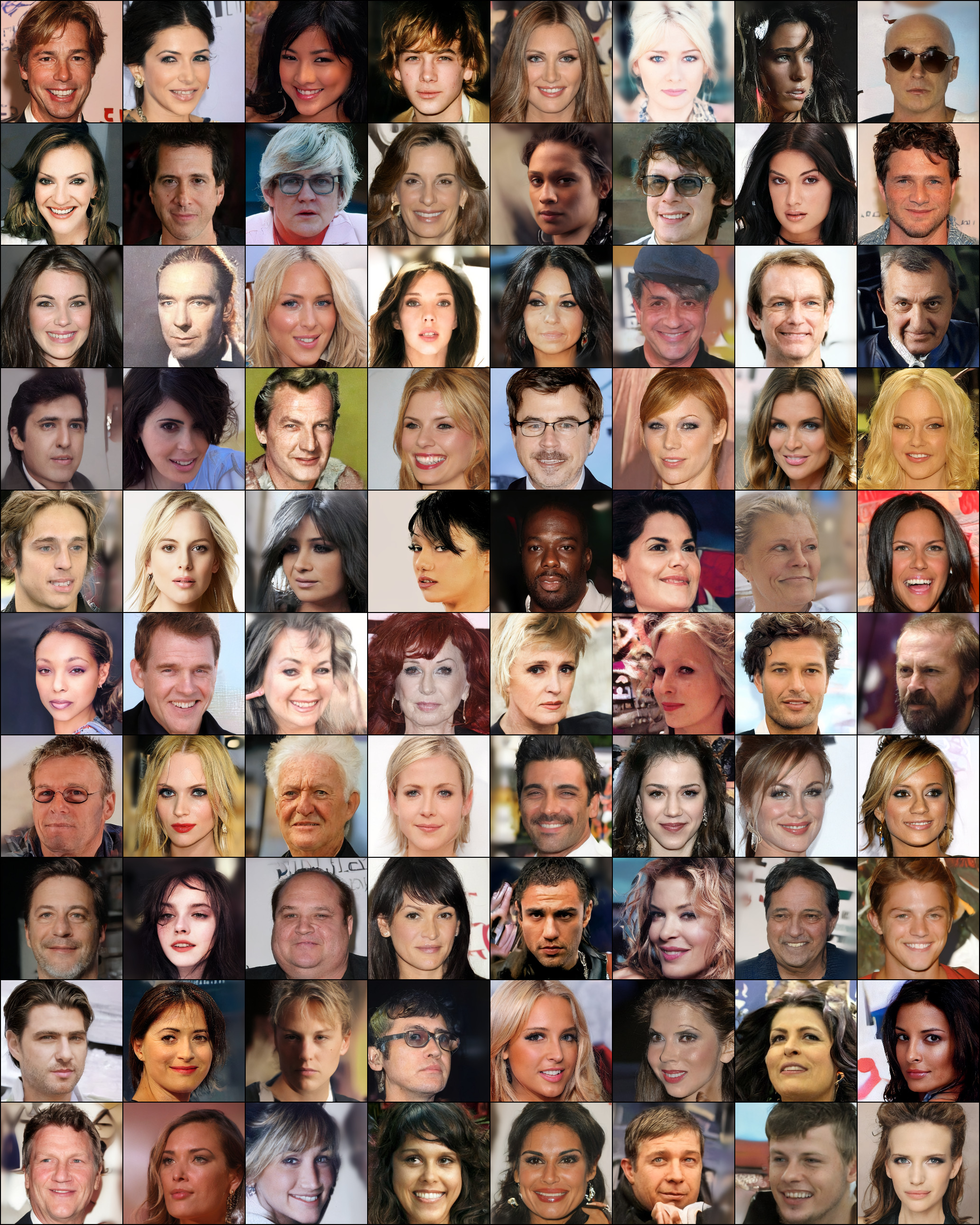
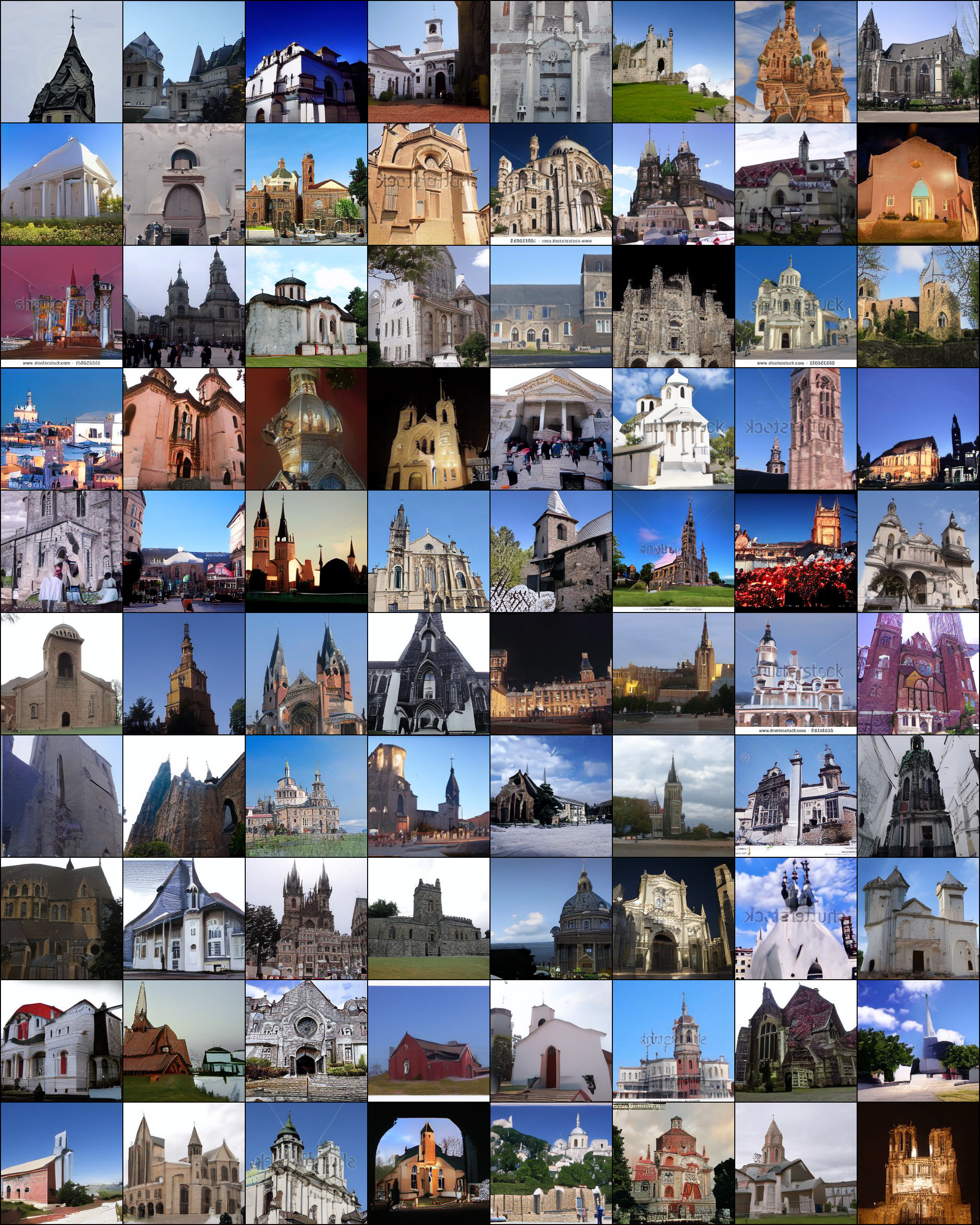
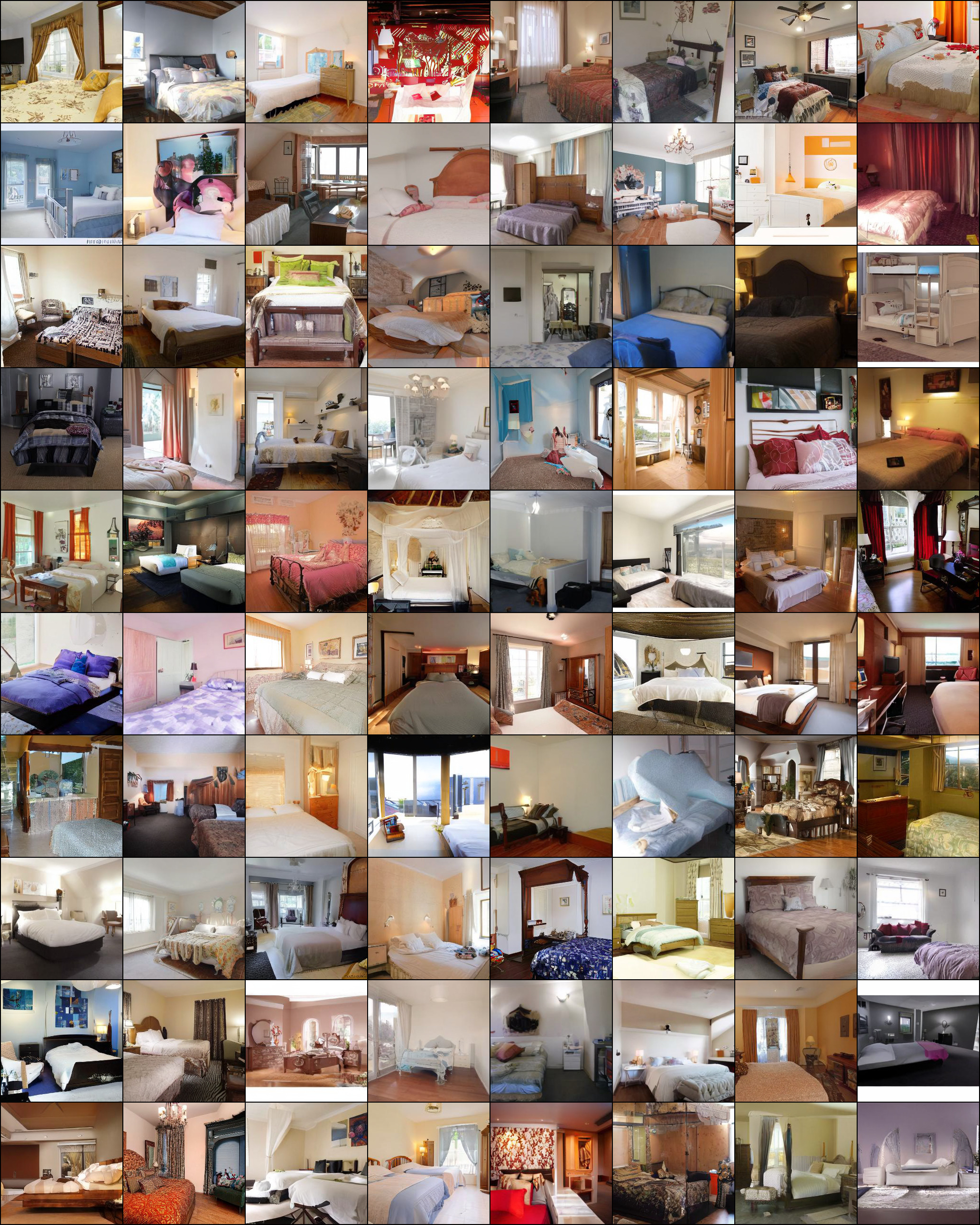
우리는 다음의 unconditional models를 학습한다${256}^2$CelebA-HQ의 images[39], FFHQ[41], LSUN-Churches 및-Bedrooms [102]그리고 i) sample quality 및 ii) data manifold에 대한 그것들의 coverage를 ii) FID를 사용하여 평가한다[29]및 ii) Precision-and-Recall[50]. Tab.1는 우리의 결과를 요약한다. CelebA-HQ에서, 우리는 새로운 state-of-the-art FID인$5.11$을 보고하며, 이전 likelihood-based models뿐 아니라 GANs도 능가한다. 우리는 또한 LSGM을 능가한다[93]여기서는 latent diffusion model이 first stage와 함께 공동으로 학습된다. 대조적으로, 우리는 고정된 space에서 diffusion models를 학습하고 reconstruction quality와 latent space에 대한 prior 학습 사이의 가중치를 조절하는 어려움을 피한다, Fig. 참조1-2.

우리는 LSUN-Bedrooms dataset을 제외한 모든 dataset에서 이전 diffusion 기반 접근법을 능가하며, LSUN-Bedrooms에서는 우리의 score가 ADM에 가깝다[15], 그 parameters의 절반을 사용하고 4배 적은 train resources를 필요로 함에도 불구하고 (Appendix 참조E.3.5). 더욱이,LDMs는 Precision 및 Recall에서 GAN-based methods보다 일관되게 향상되어, adversarial approaches에 비해 mode-covering likelihood-based training objective의 장점을 확인한다. Fig.4에서 우리는 또한 각 dataset에 대한 qualitative results를 보인다.

4.3 조건부 Latent Diffusion

Figure 8: 다음을 사용한 layout-to-image synthesisLDMon COCO[4], Sec. 참조4.3.1. 정량적 평가는 supplement에 있음D.3.

4.3.1 LDMs를 위한 Transformer Encoders

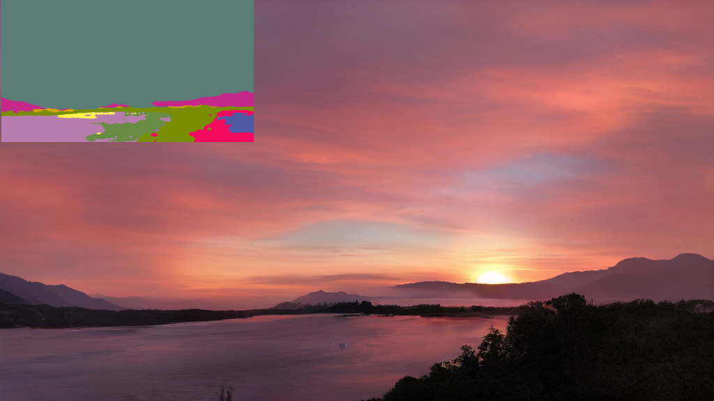
cross-attention 기반 conditioning을 LDMs에 도입함으로써 우리는 diffusion models에서 이전에는 탐구되지 않았던 다양한 conditioning modalities에 그것들을 열어 둔다. 다음을 위해text-to-imageimage modeling, 우리는 1.45B parameterKL-정규화된LDM을 LAION-400M의 language prompts에 conditioned하여 학습한다[78]. 우리는 BERT-tokenizer를 사용한다[14]그리고 구현한다${\tau }_{\theta }$transformer로서[97]latent code를 추론하기 위해, 이는 (multi-head) cross-attention을 통해 UNet에 매핑된다 (Sec.3.3). language representation 학습과 visual synthesis를 위한 domain specific experts의 이 조합은 강력한 모델을 낳으며, 복잡한 user-defined text prompts에 잘 일반화된다,cf.Fig.8및5. 정량적 분석을 위해, 우리는 prior work를 따르고 MS-COCO에서 text-to-image generation을 평가한다[51]validation set, 여기서 우리의 모델은 강력한 AR[66, 17]및 GAN-based[109]methods를 개선한다,cf.Tab.2. 우리는 classifier-free diffusion guidance를 적용하는 것이[32]sample quality를 크게 향상시켜, guidedLDM-KL-8-G가 최근 state-of-the-art AR[26]및 diffusion models와 동등한 수준이 되도록 한다는 점에 주목한다[59]text-to-image synthesis에 대해, parameter count를 상당히 줄이면서도 그렇다. cross-attention 기반 conditioning mechanism의 유연성을 더 분석하기 위해, 우리는 또한 다음에 기반해 이미지를 합성하는 models를 학습한다semantic layoutson OpenImages[49], 그리고 COCO에서 finetune한다[4], Fig. 참조8. Sec. 참조D.3정량적 평가와 구현 세부사항을 위해.

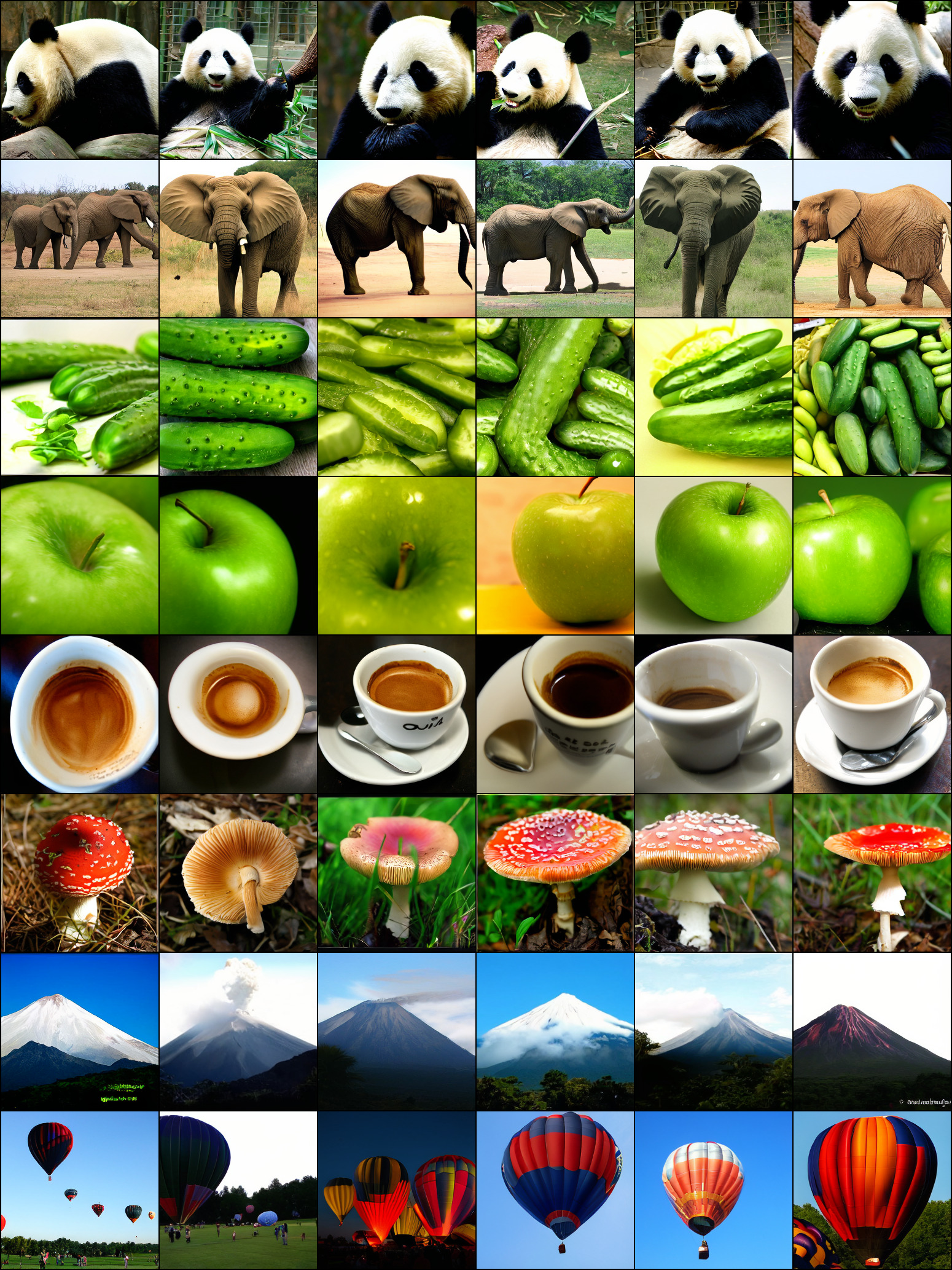
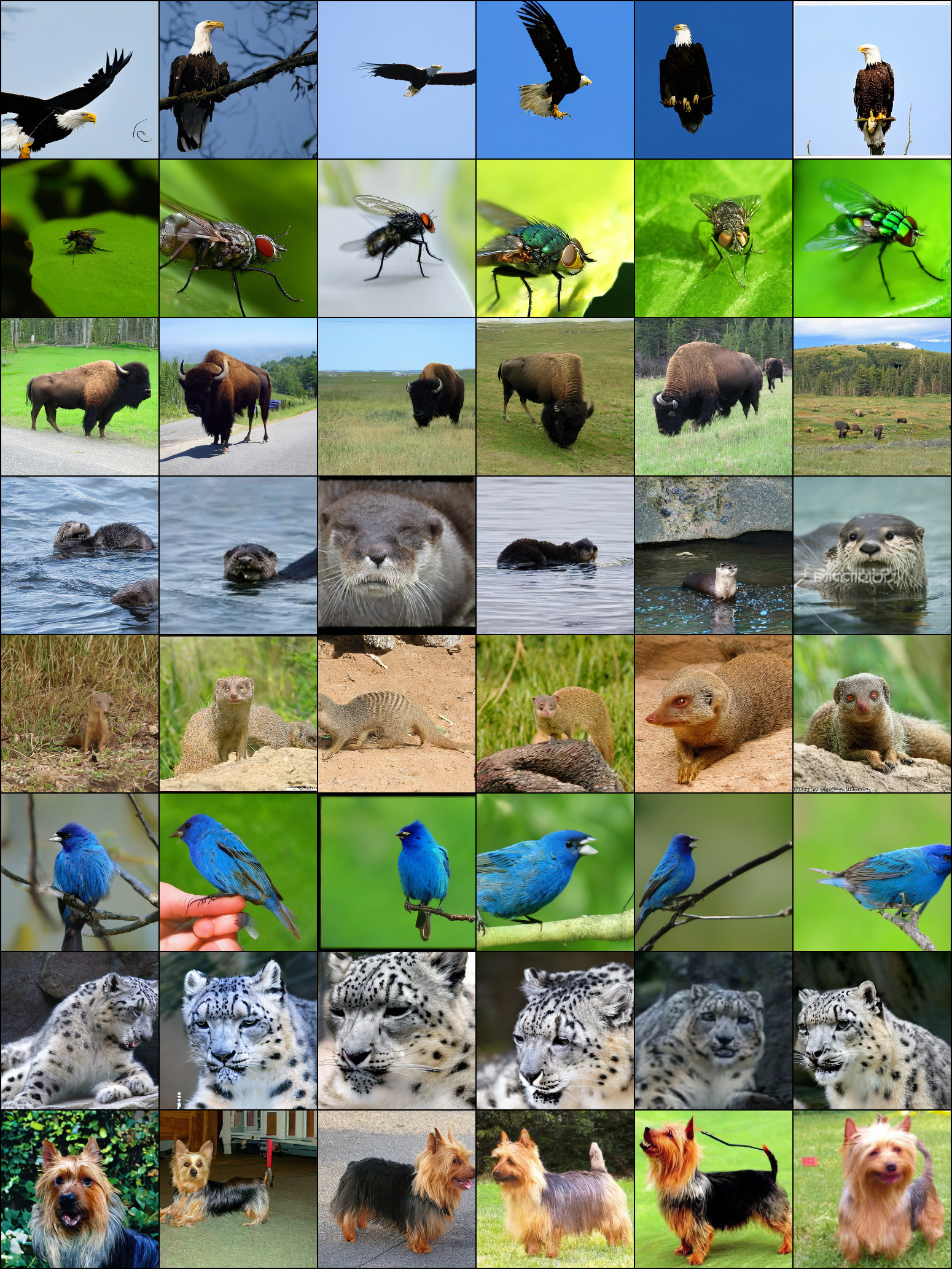
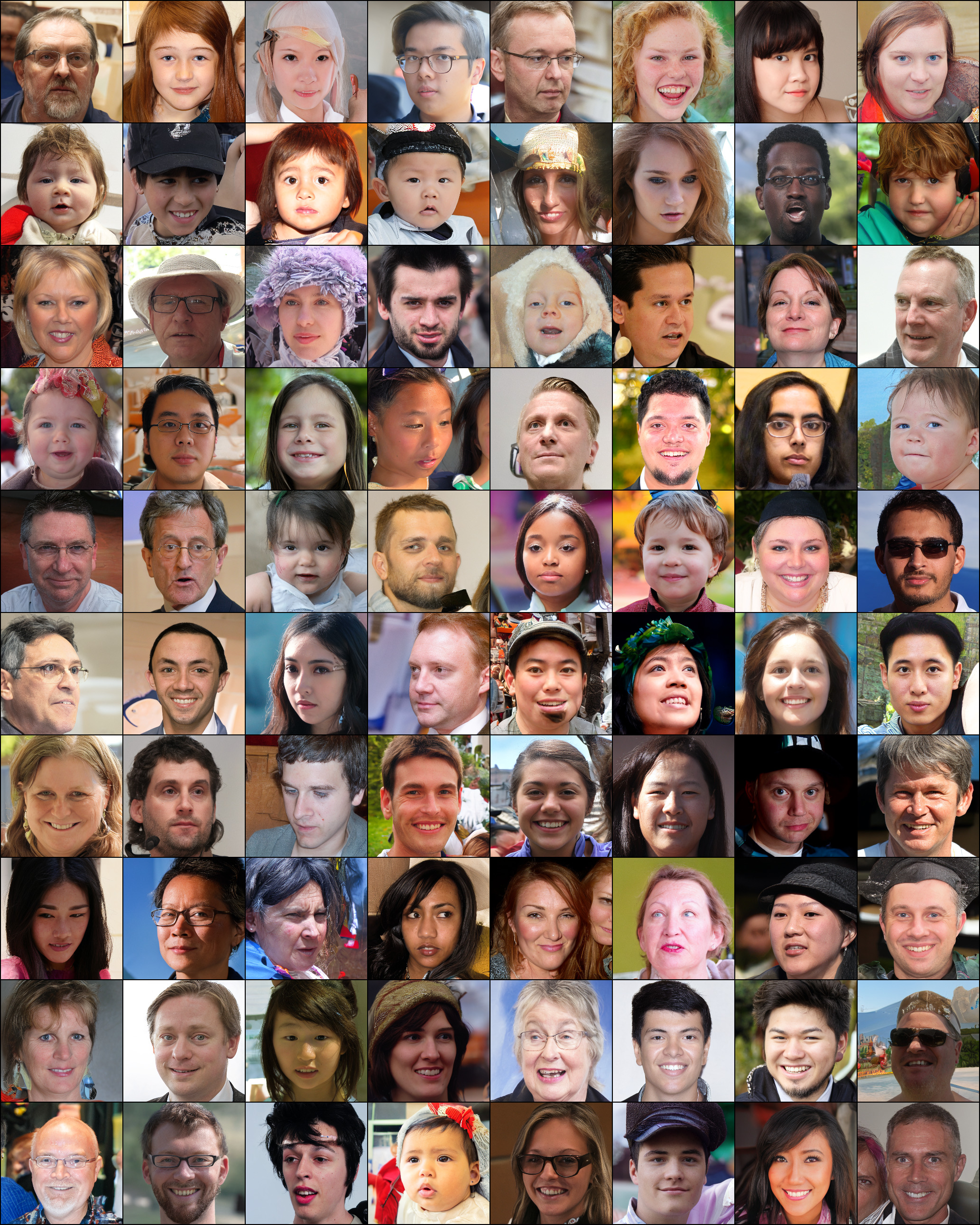
마지막으로, prior work를 따라[15, 3, 23, 21], 우리는 가장 성능이 좋은 우리의class-conditionalImageNet models를 평가한다$f\in \{4,8\}$Sec.의4.1Tab.에서3, Fig.4및 Sec.D.4. 여기서 우리는 state of the art diffusion model ADM을 능가한다[15]계산 요구량과 parameter count를 상당히 줄이면서,cf.Tab18.

방법 FID$\downarrow$ IS$\uparrow$ Precision$\uparrow$ Recall$\uparrow$ $N_{\text{params}}$ BigGan-deep[3] 6.95 203.6$\pm \text{2.6}$ 0.87 0.28 340M - ADM[15] 10.94 100.98 0.69 0.63 554M 250 DDIM steps ADM-G[15] 4.59 186.7 0.82 0.52 608M 250 DDIM steps LDM-4(ours) 10.56 103.49$\pm \text{1.24}$ 0.71 0.62 400M 250 DDIM steps LDM-4-G (ours) 3.60 247.67$\pm \text{5.59}$ 0.87 0.48 400M 250 steps, c.f.g[32], $s=1.5$

Table 3: class-conditional ImageNet의 비교LDMImageNet에서 class-conditional image generation을 위한 최근 state-of-the-art methods와[12]. 추가 baselines를 포함한 더 자세한 비교는 다음에서 찾을 수 있다D.4, Tab.10및F. c.f.g.는 scale을 가진 classifier-free guidance를 나타낸다$s$다음에서 제안된 바와 같이[32].

4.3.2 Beyond를 넘어서는 Convolutional Sampling${256}^2$

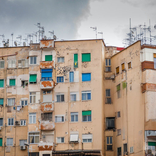
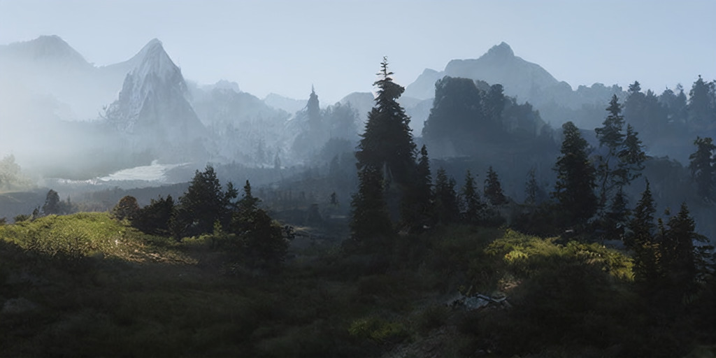
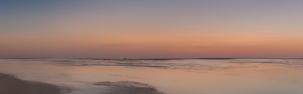
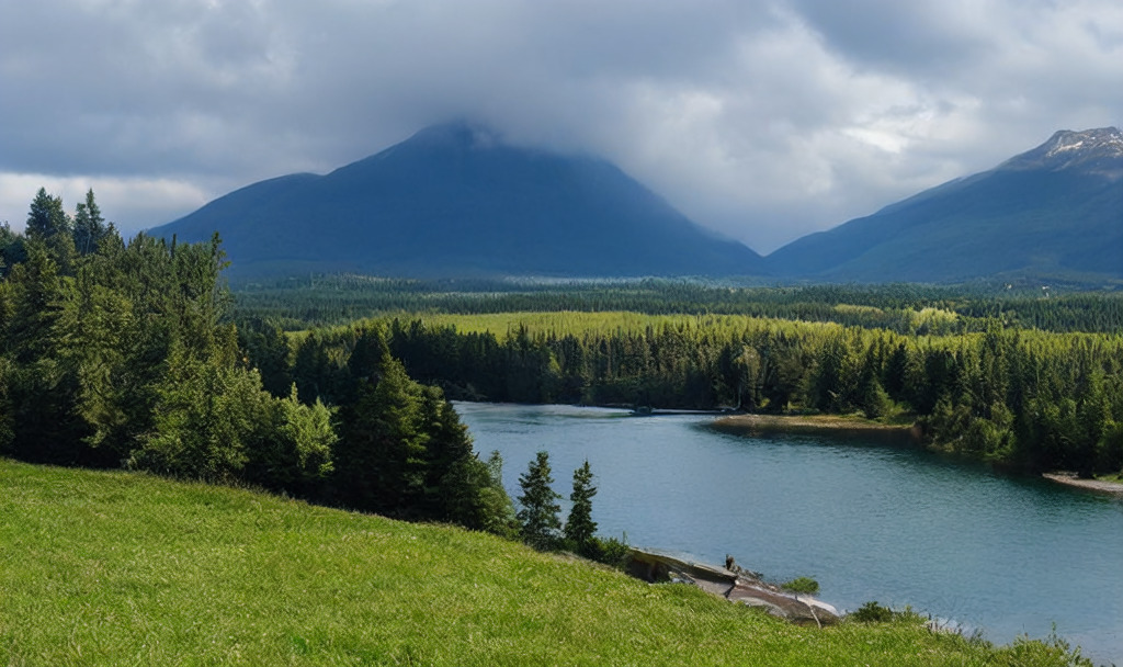
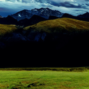
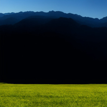
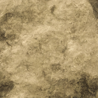
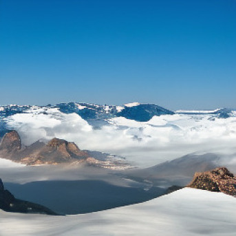
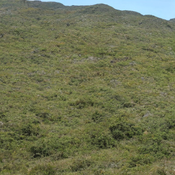
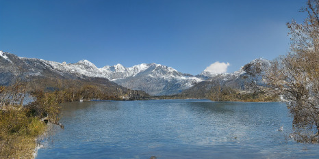
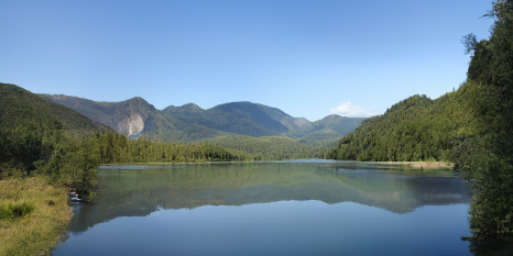
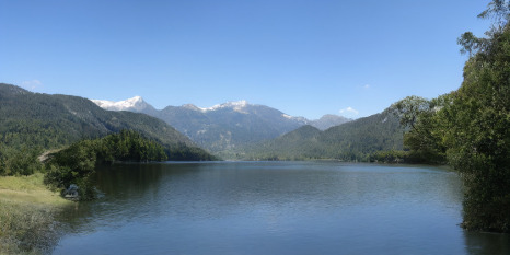
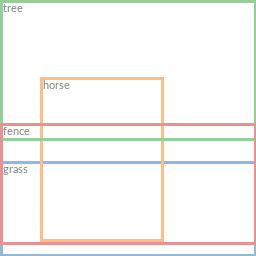
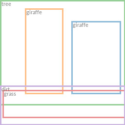
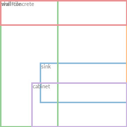
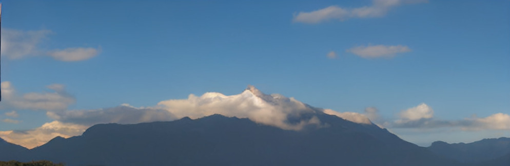
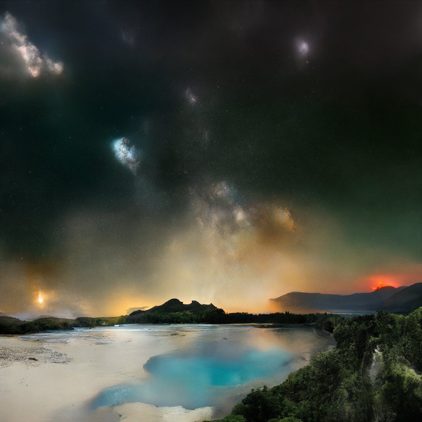
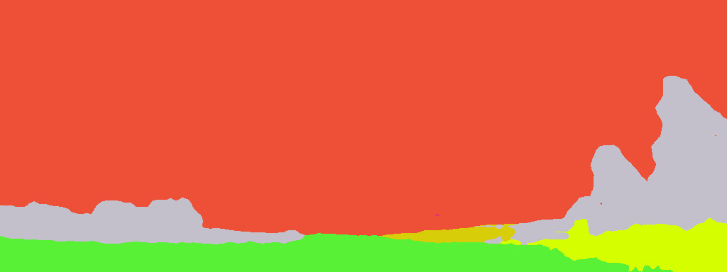
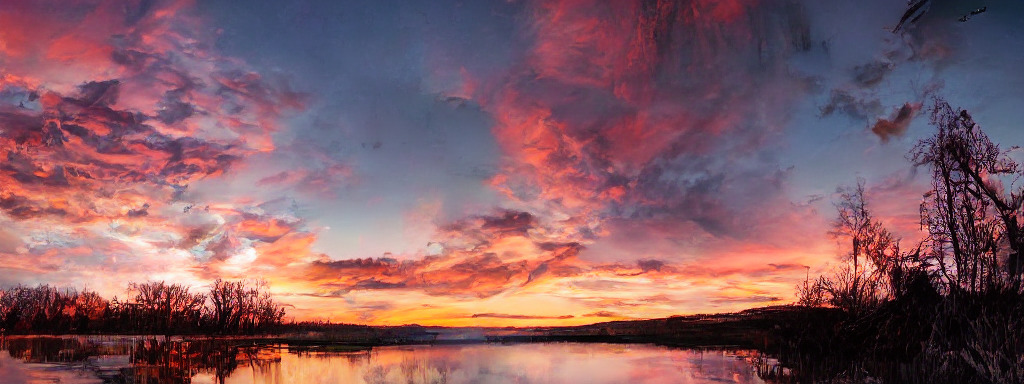
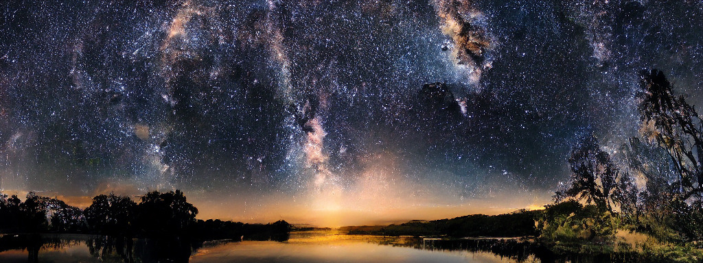
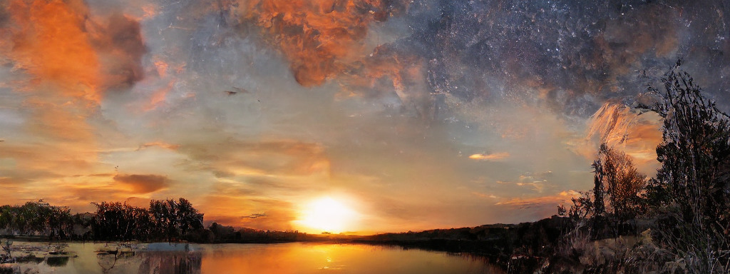
spatially aligned conditioning information을 입력에 concatenate함으로써${ϵ}_{\theta }$, LDMs는 효율적인 general-purpose image-to-image translation models로 기능할 수 있다. 우리는 이를 사용해 semantic synthesis, super-resolution (Sec.4.4) 및 inpainting (Sec.4.5)을 위한 models를 학습한다. semantic synthesis를 위해, 우리는 semantic maps와 paired된 landscapes images를 사용한다[61, 23]그리고 semantic maps의 downsampled versions를 다음의 latent image representation과 concatenate한다$f=4$model (VQ-reg., Tab. 참조8). 우리는 input resolution에서 학습한다${256}^2$(다음에서의 crops${384}^2$) 그러나 우리의 모델이 더 큰 resolutions로 일반화되며 convolutional 방식으로 평가될 때 megapixel regime까지 images를 생성할 수 있음을 발견한다 (Fig. 참조9). 우리는 이 behavior를 활용해 Sec.의 super-resolution models도 적용한다4.4및 Sec.의 inpainting models4.5사이의 큰 images를 생성하기 위해${512}^2$및${1024}^2$. 이 application의 경우, signal-to-noise ratio (latent space의 scale에 의해 유도됨)가 결과에 상당한 영향을 미친다. Sec.D.1에서 우리는 (i) 다음에 의해 제공되는 latent space에서 LDM을 학습할 때 이를 설명한다$f=4$model (KL-reg., Tab. 참조8), 그리고 (ii) component-wise standard deviation에 의해 scaled된 rescaled version.

후자는 classifier-free guidance와 결합하여[32], 또한 다음의 직접 합성을 가능하게 한다$>{256}^2$text-conditional을 위한 imagesLDM-KL-8-GFig.에서와 같이13.

Figure 9: A LDM에서 학습된${256}^2$resolution은 더 큰 resolution으로 일반화될 수 있다 (여기서는:$512\times 1024$) landscape images의 semantic synthesis와 같은 spatially conditioned tasks에 대해. Sec. 참조4.3.2.

4.4 Latent Diffusion을 사용한 Super-Resolution

LDMs는 concatenation을 통해 low-resolution images에 직접 conditioning함으로써 super-resolution을 위해 효율적으로 학습될 수 있다 (cf.Sec.3.3). 첫 번째 experiment에서, 우리는 SR3를 따른다[72]그리고 image degradation을 bicubic interpolation with로 고정한다$4\times$-downsampling 그리고 SR3의 data processing pipeline을 따라 ImageNet에서 학습한다. 우리는 다음을 사용한다$f=4$OpenImages에서 pretrained된 autoencoding model (VQ-reg.,cf.Tab.8) 그리고 low-resolution conditioning을 concatenate한다$y$및 UNet에 대한 inputs,i.e. ${\tau }_{\theta }$는 identity이다. 우리의 qualitative 및 quantitative results (Fig. 참조10및 Tab.5)는 competitive performance를 보이며 LDM-SR은 FID에서 SR3를 능가하는 반면 SR3는 더 나은 IS를 가진다. 단순한 image regression model은 가장 높은 PSNR 및 SSIM scores를 달성하지만, 이러한 metrics는 human perception과 잘 일치하지 않는다[106]그리고 imperfectly aligned high frequency details보다 blurriness를 선호한다[72]. 또한, 우리는 pixel-baseline과 LDM-SR을 비교하는 user study를 수행한다. 우리는 SR3를 따른다[72]여기서 human subjects는 두 high-res images 사이에 low-res image를 보여 받았고 preference를 질문받았다. Tab.의 결과는4LDM-SR의 좋은 performance를 확인한다. PSNR 및 SSIM은 post-hoc guiding mechanism을 사용해 높일 수 있다[15]그리고 우리는 이를 구현한다image-based guiderperceptual loss를 통해, Sec. 참조D.6.

bicubic	LDM-SR	SR3

Figure 10: ImageNet 64$\to$256 super-resolution on ImageNet-Val.LDM-SR는 realistic textures를 rendering하는 데 장점이 있지만 SR3는 더 coherent한 fine structures를 합성할 수 있다. 추가 samples와 cropouts는 appendix를 참조하라. SR3 results는 다음에서 가져옴[72].

SR on ImageNet Inpainting on Places User Study Pixel-DM ($f1$) LDM-4 LAMA[88] LDM-4 Task 1:Preference vs GT$\uparrow$ 16.0% 30.4% 13.6% 21.0% Task 2:Preference Score$\uparrow$ 29.4% 70.6% 31.9% 68.1%

Table 4: Task 1: Subjects에게 ground truth와 generated image를 보여 주고 preference를 물었다. Task 2: Subjects는 두 generated images 중 하나를 결정해야 했다. 더 자세한 내용은 다음에 있음E.3.6

bicubic degradation process는 이 pre-processing을 따르지 않는 images에는 잘 일반화되지 않기 때문에, 우리는 또한 generic model을 학습한다,LDM-BSR, 더 다양한 degradation을 사용하여. 결과는 Sec.에 제시되어 있다D.6.1.

방법 FID$\downarrow$ IS$\uparrow$ PSNR$\uparrow$ SSIM$\uparrow$ $N_{\text{params}}$ $\left[\frac{\text{samples}}{s}\right]{(}^{\ast })$ 이미지 회귀[72] 15.2 121.1 27.9 0.801 625M N/A SR3[72] 5.2 180.1 26.4 0.762 625M N/A LDM-4(우리의 것, 100 steps) 2.8^†/4.8^‡ 166.3 24.4$\pm$3.8 0.69$\pm$0.14 169M 4.62 emphLDM-4 (우리의 것, big, 100 steps) 2.4^†/4.3^‡ 174.9 24.7$\pm$4.1 0.71$\pm$0.15 552M 4.5 LDM-4(우리의 것, 50 steps, guiding) 4.4^†/6.4^‡ 153.7 25.8$\pm$3.7 0.74$\pm$0.12 184M 0.38

Table 5: $\times 4$ImageNet-Val에서의 업스케일링 결과. (${256}^2$); ^†: validation split에서 계산된 FID features,^‡: train split에서 계산된 FID features;^∗: NVIDIA A100에서 평가됨

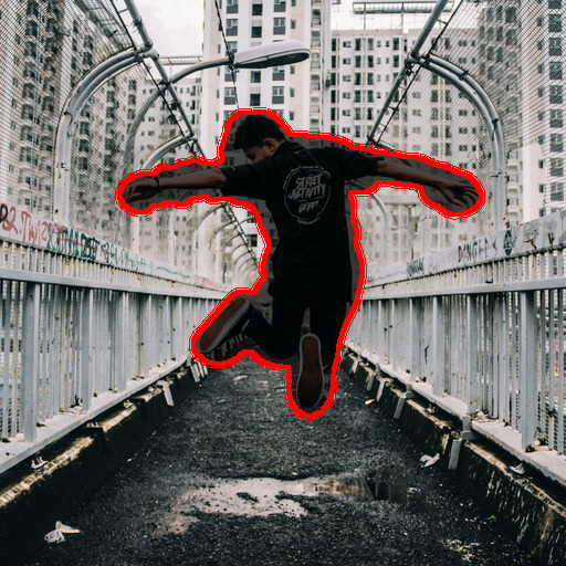
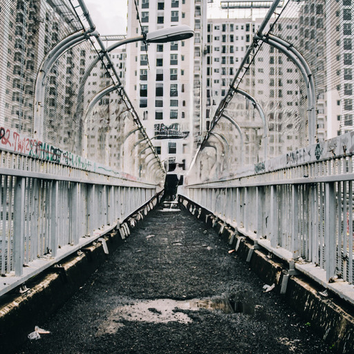
4.5 Latent Diffusion을 사용한 Inpainting

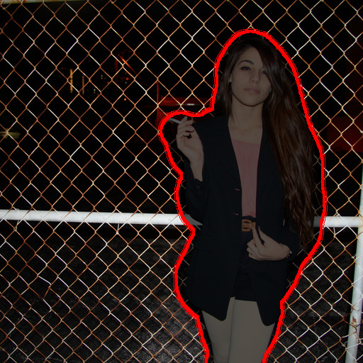
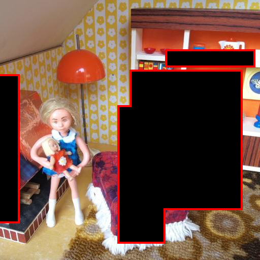
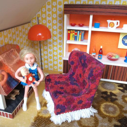
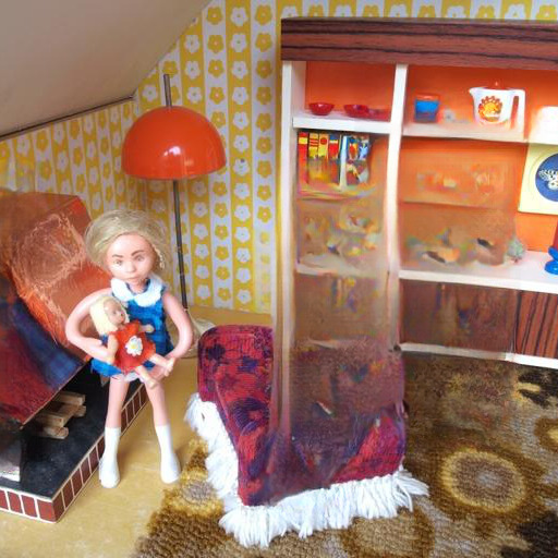
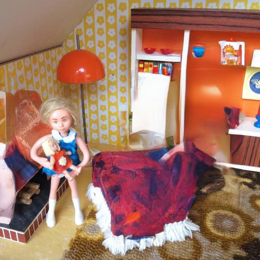
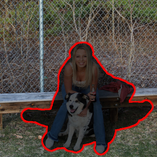
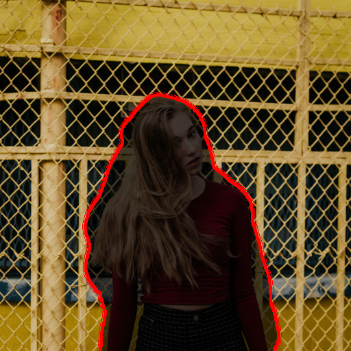
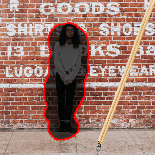
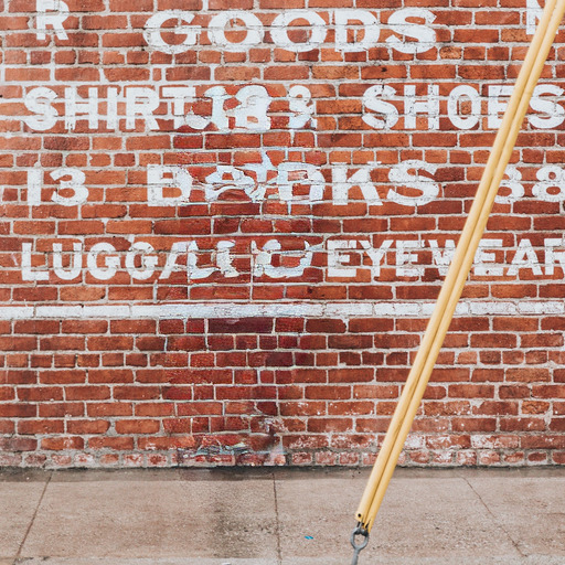
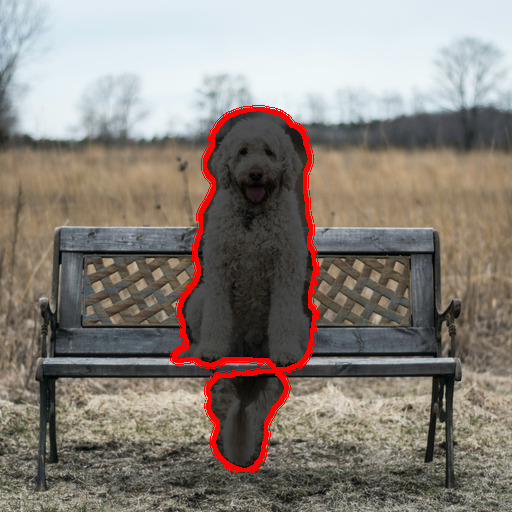
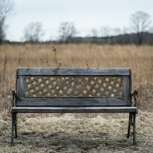
Inpainting은 이미지의 일부가 손상되었거나 이미지 내의 기존이지만 원치 않는 내용을 대체하기 위해 이미지의 마스크된 영역을 새로운 콘텐츠로 채우는 작업이다. 우리는 조건부 이미지 생성을 위한 우리의 일반적 접근법이 이 작업을 위한 더 전문화된 최신 접근법들과 어떻게 비교되는지 평가한다. 우리의 평가는 LaMa의 프로토콜을 따른다[88], Fast Fourier Convolutions에 의존하는 특수한 아키텍처를 도입한 최근의 inpainting 모델[8]. 정확한 훈련&Places에서의 평가 프로토콜[108]은 Sec.에 설명되어 있다E.2.2.

우리는 먼저 첫 번째 단계에 대한 서로 다른 설계 선택의 효과를 분석한다.

train throughput sampling throughput^† train+val FID@2k Model (reg.-type) samples/sec. @256 @512 hours/epoch epoch 6 LDM-1(no first stage) 0.11 0.26 0.07 20.66 24.74 LDM-4 (KL, w/ attn) 0.32 0.97 0.34 7.66 15.21 LDM-4 (VQ, w/ attn) 0.33 0.97 0.34 7.04 14.99 LDM-4 (VQ, w/o attn) 0.35 0.99 0.36 6.66 15.95

Table 6: inpainting 효율성 평가.^†: Fig.와의 차이7는 다양한 GPU 설정/batch sizes 때문이다cf.supplement.

입력	결과

Figure 11: 우리의 모델을 사용한 객체 제거의 정성적 결과big, w/ ftinpainting 모델. 더 많은 결과는 Fig.를 보라22.

특히, 우리는 inpainting 효율성을 비교한다LDM-1 (i.e.픽셀 기반 조건부 DM)과LDM-4, 둘 다에 대해KL및VQregularizations, 그리고VQ-LDM-4첫 번째 단계에 attention이 전혀 없는 경우( Tab. 참조8), 여기서 후자는 고해상도에서 디코딩을 위한 GPU 메모리를 줄인다. 비교 가능성을 위해, 우리는 모든 모델의 파라미터 수를 고정한다. Tab.6는 resolution에서의 training 및 sampling throughput을 보고한다${256}^2$및${512}^2$, epoch당 총 훈련 시간(시간)과 6 epochs 후 validation split에서의 FID score. 전반적으로, 우리는 적어도 다음의 speed-up을 관찰한다$2.7\times$픽셀 기반 diffusion models와 latent 기반 diffusion models 사이에서, FID scores를 적어도 다음 배수만큼 개선하면서$1.6\times$.

Tab.의 다른 inpainting 접근법과의 비교7는 attention을 사용한 우리의 모델이 FID로 측정한 전체 이미지 품질을 다음보다 개선함을 보여준다[88]. 마스크되지 않은 이미지와 우리의 samples 사이의 LPIPS는 다음보다 약간 더 높다[88]. 우리는 이것을 다음에 기인한다고 본다[88]단 하나의 결과만 생성하여 우리의 LDM이 생성한 다양한 결과와 비교해 더 평균적인 이미지를 더 많이 복원하는 경향이 있음cf.Fig.21. 추가로 사용자 연구( Tab.4)에서 인간 피험자들은 우리의 결과를 다음의 결과보다 선호한다[88].

이러한 초기 결과에 기반하여, 우리는 또한 더 큰 diffusion model (bigin Tab.7)을 다음의 latent space에서 훈련했다VQ-regularized first stage without attention. 다음을 따라[15], 이 diffusion model의 UNet은 feature hierarchy의 세 수준에서 attention layers, up- 및 downsampling을 위한 BigGAN[3]residual block을 사용하며 215M 대신 387M parameters를 가진다. 훈련 후, 우리는 resolutions에서 생성된 samples의 품질에 불일치를 발견했다${256}^2$및${512}^2$, 우리는 이것이 추가적인 attention modules에 의해 야기된 것으로 가정한다. 그러나 resolution에서 half an epoch 동안 모델을 fine-tuning하면${512}^2$모델이 새로운 feature statistics에 적응할 수 있게 하고 image inpainting에서 새로운 state of the art FID를 설정한다 (big, w/o attn, w/ ftin Tab.7, Fig.11.).

40-50% masked All samples Method FID$\downarrow$ LPIPS$\downarrow$ FID$\downarrow$ LPIPS$\downarrow$ LDM-4(우리의 것, big, w/ ft) 9.39 0.246$\pm$ 0.042 1.50 0.137$\pm$ 0.080 LDM-4(우리의 것, big, w/o ft) 12.89 0.257$\pm$ 0.047 2.40 0.142$\pm$ 0.085 LDM-4(우리의 것, w/ attn) 11.87 0.257$\pm$ 0.042 2.15 0.144$\pm$ 0.084 LDM-4(우리의 것, w/o attn) 12.60 0.259$\pm$ 0.041 2.37 0.145$\pm$ 0.084 LaMa[88]^† 12.31 0.243$\pm$ 0.038 2.23 0.134$\pm$ 0.080 LaMa[88] 12.0 0.24$\pm$ 0.000 2.21 0.14$\pm$ 0.000 CoModGAN[107] 10.4 0.26$\pm$ 0.000 1.82 0.15$\pm$ 0.000 RegionWise[52] 21.3 0.27$\pm$ 0.000 4.75 0.15$\pm$ 0.000 DeepFill v2[104] 22.1 0.28$\pm$ 0.000 5.20 0.16$\pm$ 0.000 EdgeConnect[58] 30.5 0.28$\pm$ 0.000 8.37 0.16$\pm$ 0.000

Table 7: 크기가 다음인 30k crops에서의 inpainting 성능 비교$512\times 512$Places의 test images로부터[108]. 열40-50%은 이미지 영역의 40-50%를 inpaint해야 하는 어려운 examples에 대해 계산된 metrics를 보고한다.^†원래 사용된 test set이[88]사용 가능하지 않았기 때문에, 우리의 test set에서 재계산됨.

5 한계&사회적 영향

한계

LDMs는 픽셀 기반 접근법과 비교하여 계산 요구량을 크게 줄이지만, 그들의 순차적 sampling process는 여전히 GANs보다 느리다. 더욱이, 높은 정밀도가 요구될 때 LDMs의 사용은 의문시될 수 있다: 비록 우리의$f=4$autoencoding models( Fig. 참조1)에서 이미지 품질 손실은 매우 작지만, 그것들의 reconstruction capability는 pixel space에서 세밀한 정확도를 요구하는 작업의 병목이 될 수 있다. 우리는 우리의 superresolution models (Sec.4.4)이 이미 이 점에서 어느 정도 제한되어 있다고 가정한다.

사회적 영향

이미지와 같은 미디어를 위한 generative models는 양날의 검이다: 한편으로, 그것들은 다양한 창의적 응용을 가능하게 하며, 특히 training 및 inference 비용을 줄이는 우리와 같은 접근법은 이 기술에 대한 접근을 촉진하고 그 탐구를 민주화할 잠재력이 있다. 다른 한편으로, 이는 조작된 데이터를 만들고 전파하거나 misinformation 및 spam을 퍼뜨리는 것이 더 쉬워진다는 뜻이기도 하다. 특히, 이미지의 의도적 조작(“deep fakes”)은 이 맥락에서 흔한 문제이며, 특히 여성들이 이에 의해 불균형적으로 영향을 받는다[13, 24].

Generative models는 또한 그들의 training data를 드러낼 수 있다[5, 90], 이는 데이터가 민감하거나 개인적인 정보를 포함하고 명시적 동의 없이 수집되었을 때 큰 우려가 된다. 그러나 이것이 이미지의 DMs에도 어느 정도 적용되는지는 아직 완전히 이해되지 않았다.

마지막으로, deep learning modules는 데이터에 이미 존재하는 biases를 재현하거나 악화시키는 경향이 있다[91, 38, 22]. Diffusion models는 다음보다 데이터 분포를 더 잘 포괄하지만e.g.GAN-based approaches, adversarial training과 likelihood-based objective를 결합하는 우리의 two-stage approach가 데이터를 어느 정도 잘못 표현하는지는 여전히 중요한 연구 질문으로 남아 있다.

deep generative models의 윤리적 고려사항에 대한 더 일반적이고 자세한 논의는 다음을 보라e.g. [13].

6 결론

우리는 denoising diffusion models의 품질을 저하시키지 않으면서 training 및 sampling 효율성을 모두 크게 개선하는 단순하고 효율적인 방법인 latent diffusion models를 제시했다. 이를 바탕으로, 그리고 우리의 cross-attention conditioning mechanism을 통해, 우리의 실험은 task-specific architectures 없이 광범위한 조건부 image synthesis tasks 전반에서 state-of-the-art methods와 비교해 유리한 결과를 입증할 수 있었다.

부록

Figure 12: Sec.에서와 같은 semantic landscapes 모델의 합성곱 샘플4.3.2, 에서 finetune됨${512}^2$이미지.

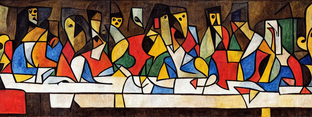
’피카소가 그린 최후의 만찬 그림.’
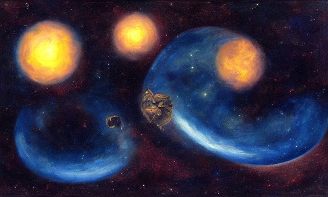
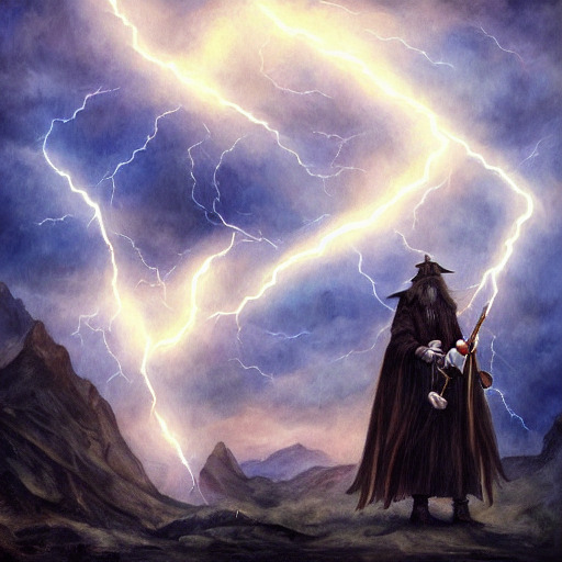
’latent space의 유화.’	’Gandalf the Black의 장대한 그림 산에서 천둥과 번개를 소환하는 중.’
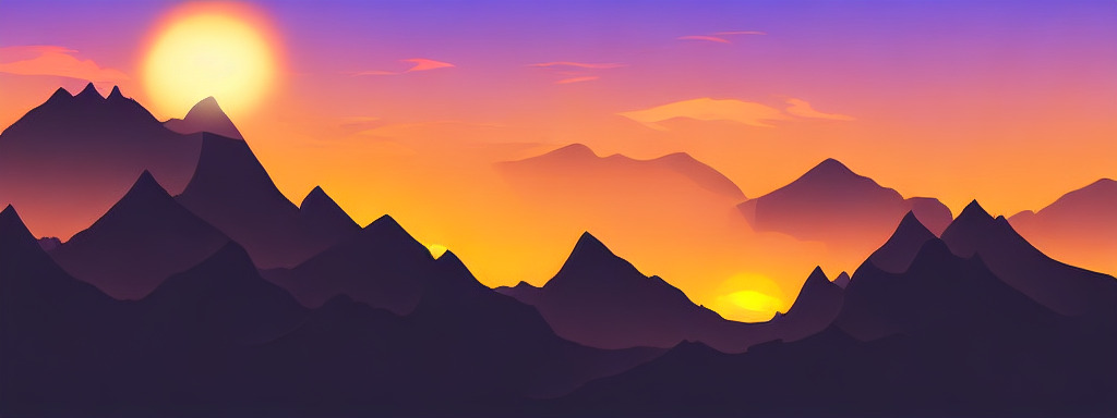
’산맥 위의 일몰, vector image.’

Figure 13: Sec.의 convolutional sampling 전략과 classifier free diffusion guidance를 결합하면4.3.2, 우리의 1.45B parameter text-to-image model은 native보다 더 큰 이미지를 렌더링하는 데 사용될 수 있다${256}^2$모델이 학습된 resolution.

Appendix AChangelog

여기서는 이 버전(https://arxiv.org/abs/2112.10752v2)의 논문과 이전 버전 사이의 변경 사항을 나열한다,i.e. https://arxiv.org/abs/2112.10752v1.

• 우리는 Sec.의 text-to-image synthesis 결과를 업데이트했다4.3이는 새롭고 더 큰 모델(1.45B parameters)을 학습하여 얻은 것이다. 여기에는 또한 우리의 작업이 발표된 것과 같은 시점에([59, 109]) 또는 이후에([26]) arXiv에 발표된 이 과제에 대한 매우 최근의 경쟁 방법들과의 새로운 비교도 포함된다.

• 우리는 Sec.의 ImageNet에서 class-conditional synthesis 결과를 업데이트했다4.1, Tab.3(Sec.도 참조D.4) 이는 더 큰 batch size로 모델을 재학습하여 얻은 것이다. Fig.의 해당 정성적 결과26및 Fig.27도 업데이트되었다. 업데이트된 text-to-image와 class-conditional model 둘 다 이제 classifier-free guidance를 사용한다[32]시각적 충실도를 높이기 위한 조치로.

• 우리는 user study를 수행했다(Saharia et al가 제안한 방식에 따라[72]) 이는 우리의 inpainting(Sec.4.5) 및 superresolution models(Sec.4.4).

• Fig.를 추가했다5본문에, Fig.를 옮겼다18appendix로, Fig.를 추가했다13appendix에.

Appendix BDenoising Diffusion Models에 대한 상세 정보

Diffusion models는 signal-to-noise ratio의 관점에서 지정될 수 있다$\text{SNR}\left(t\right)=\frac{{\alpha }_t^2}{{\sigma }_t^2}$sequences로 구성되는${\left({\alpha }_t\right)}_{t=1}^T$그리고${\left({\sigma }_t\right)}_{t=1}^T$이는 data sample에서 시작하여$x_0$, forward diffusion process를 정의한다$q$다음과 같이

$q\left(x_t|x_0\right)=𝒩\left(x_t|{\alpha }_t{x}_0,{\sigma }_t^2𝕀\right)$ (4)

에 대한 Markov structure와 함께:

$q\left(x_t|x_s\right)$ $=𝒩\left(x_t|{\alpha }_{t|s}{x}_s,{\sigma }_{t|s}^2𝕀\right)$ (5)

${\alpha }_{t|s}$ $=\frac{{\alpha }_t}{{\alpha }_s}$ (6)

${\sigma }_{t|s}^2$ $={\sigma }_t^2-{\alpha }_{t|s}^2{\sigma }_s^2$ (7)

Denoising diffusion models는 generative models이다$p\left(x_0\right)$이는 이 과정을 시간상 뒤로 진행되는 유사한 Markov structure로 되돌리며,i.e.다음과 같이 지정된다

$p\left(x_0\right)={\int }_{z}p\left(x_T\right)\prod _{t=1}^{T}p\left(x_{t-1}|x_t\right)$ (8)

이 모델과 관련된 evidence lower bound (ELBO)는 그런 다음 discrete time steps에 걸쳐 다음과 같이 분해된다

$-\log p\left(x_0\right)\le 𝕂𝕃\left(q\left(x_T\right|x_0)\right|p\left(x_T\right))+\sum _{t=1}^T{𝔼}_{q\left(x_t|x_0\right)}𝕂𝕃\left(q\left(x_{t-1}\right|x_t,x_0)\right|p\left(x_{t-1}\right|x_t))$ (9)

prior$p\left(x_T\right)$는 일반적으로 standard normal distribution으로 선택되며, ELBO의 첫 번째 항은 그때 최종 signal-to-noise ratio에만 의존한다$\text{SNR}\left(T\right)$. 남은 항들을 최소화하기 위해, 를 parameterize하는 일반적인 선택은$p\left(x_{t-1}|x_t\right)$그것을 true posterior의 관점에서 지정하는 것이다$q\left(x_{t-1}|x_t,x_0\right)$하지만 알려지지 않은$x_0$를 추정값으로 대체하여$x_{\theta }(x_t,t)$현재 step에 기반한$x_t$. 이는 다음을 준다[45]

$p\left(x_{t-1}|x_t\right)$ $≔q\left(x_{t-1}|x_t,x_{\theta }(x_t,t)\right)$ (10)

$=𝒩\left(x_{t-1}|{\mu }_{\theta }(x_t,t),{\sigma }_{t|t-1}^2\frac{{\sigma }_{t-1}^2}{{\sigma }_t^2}𝕀\right),$ (11)

여기서 mean은 다음과 같이 표현될 수 있다

${\mu }_{\theta }(x_t,t)=\frac{{\alpha }_{t|t-1}{\sigma }_{t-1}^2}{{\sigma }_t^2}{x}_t+\frac{{\alpha }_{t-1}{\sigma }_{t|t-1}^2}{{\sigma }_t^2}{x}_{\theta }(x_t,t).$ (12)

이 경우, ELBO의 합은 다음으로 단순화된다

$\sum _{t=1}^T{𝔼}_{q\left(x_t|x_0\right)}𝕂𝕃\left(q\left(x_{t-1}\right|x_t,x_0)\right|p\left(x_{t-1}\right)=\sum _{t=1}^T{𝔼}_{𝒩\left(ϵ|0,𝕀\right)}\frac{1}{2}(\text{SNR}(t-1)-\text{SNR}\left(t\right))\parallel x_0-x_{\theta }({\alpha }_t{x}_0+{\sigma }_tϵ,t){\parallel }^2$ (13)

다음을 따라[30], 우리는 reparameterization을 사용한다

${ϵ}_{\theta }(x_t,t)=\left(x_t-{\alpha }_t{x}_{\theta }(x_t,t)\right)/{\sigma }_t$ (14)

reconstruction term을 denoising objective로 표현하기 위해,

${\Vert x_0-x_{\theta }({\alpha }_t{x}_0+{\sigma }_tϵ,t)\Vert }^2=\frac{{\sigma }_t^2}{{\alpha }_t^2}{\Vert ϵ-{ϵ}_{\theta }({\alpha }_t{x}_0+{\sigma }_tϵ,t)\Vert }^2$ (15)

그리고 reweighting은 각 항에 같은 가중치를 할당하며 Eq. (1).

Appendix CImage Guiding Mechanisms

Samples${256}^2$	Guided Convolutional Samples${512}^2$	Convolutional Samples${512}^2$

Figure 14: landscapes에서, unconditional models를 사용한 convolutional sampling은 균질하고 비일관적인 global structures로 이어질 수 있다(2열 참조).$L_2$-guiding을 low resolution image와 함께 사용하면 일관된 global structures를 재확립하는 데 도움이 될 수 있다.

diffusion models의 흥미로운 특징은 unconditional models가 test-time에 conditioned될 수 있다는 것이다[85, 82, 15]. 특히,[15]ImageNet dataset에서 학습된 unconditional 및 conditional models 둘 다를 classifier로 guide하는 알고리즘을 제시했다$\log p_{\Phi }\left(y|x_t\right)$, diffusion process의 각 에 대해 학습된$x_t$. 우리는 이 formulation에 직접 기반하여 post-hoc를 도입한다image-guiding:

fixed variance를 가진 epsilon-parameterized model에 대해, 에서 도입된 guiding algorithm은[15]다음과 같다:

$\widehat{ϵ}\leftarrow {ϵ}_{\theta }(z_t,t)+\sqrt{1-{\alpha }_t^2}{\nabla }_{z_t}\log p_{\Phi }\left(y|z_t\right).$ (16)

이는 “score”를 보정하는 update로 해석될 수 있다${ϵ}_{\theta }$conditional distribution으로$\log p_{\Phi }\left(y|z_t\right)$.

지금까지 이 scenario는 single-class classification models에만 적용되었다. 우리는 guiding distribution을 재해석한다$p_{\Phi }\left(y|T\left(𝒟\left(z_0\left(z_t\right)\right)\right)\right)$target image가 주어진 general purpose image-to-image translation task로$y$, 여기서$T$는 identity, downsampling operation 또는 유사한 것과 같이 해당 image-to-image translation task에 채택된 임의의 differentiable transformation일 수 있다.
예로, fixed variance를 가진 Gaussian guider를 가정할 수 있다${\sigma }^2=1$, 그래서

$\log p_{\Phi }\left(y|z_t\right)=-\frac{1}{2}{\Vert y-T\left(𝒟\left(z_0\left(z_t\right)\right)\right)\Vert }_2^2$ (17)

는 가 된다$L_2$regression objective.

Fig.14는 이 formulation이 에서 학습된 unconditional model의 upsampling mechanism으로 어떻게 기능할 수 있는지 보여준다${256}^2$images, 여기서 size의 unconditional samples가${256}^2$의 convolutional synthesis를 guide한다${512}^2$images 그리고$T$는 이다$2\times$bicubic downsampling. 이 동기를 따라, 우리는 perceptual similarity guiding도 실험하고 를 대체한다$L_2$objective를 LPIPS로[106]metric, Sec. 참조4.4.

Appendix DAdditional Results

D.1 High-Resolution Synthesis를 위한 Signal-to-Noise Ratio 선택

KL-reg, w/o rescaling	KL-reg, w/ rescaling	VQ-reg, w/o rescaling

Figure 15: convolutional sampling에서 latent space rescaling의 효과를 설명하며, 여기서는 landscapes에 대한 semantic image synthesis의 경우이다. Sec. 참조4.3.2및 Sec.D.1.

Sec.에서 논의한 것처럼4.3.2, latent space의 variance에 의해 유도되는 signal-to-noise ratio(i.e. $\text{Var(z)}/{\sigma }_t^2$)는 convolutional sampling의 결과에 상당한 영향을 미친다. 예를 들어, KL-regularized model의 latent space에서 직접 LDM을 학습할 때(Tab. 참조8), 이 ratio는 매우 높아서 model이 reverse denoising process 초기에 많은 semantic detail을 할당한다. 반대로, Sec.에 설명된 것처럼 latents의 component-wise standard deviation으로 latent space를 rescaling하면G, SNR은 감소한다. 우리는 Fig.에서 semantic image synthesis를 위한 convolutional sampling에 미치는 효과를 설명한다15. VQ-regularized space는 에 가까운 variance를 가진다는 점에 주목하라$1$, 따라서 rescale될 필요가 없다.

D.2 모든 First Stage Models의 전체 목록

우리는 OpenImages dataset에서 학습된 다양한 autoenconding models의 완전한 목록을 Tab.에 제공한다8.

$f$ $\left|𝒵\right|$ $c$ R-FID $\downarrow$ R-IS $\uparrow$ PSNR $\uparrow$ PSIM $\downarrow$ SSIM $\uparrow$ 16 VQGAN [23] 16384 256 4.98 – 19.9 $\pm 3.4$ 1.83 $\pm 0.42$ 0.51 $\pm 0.18$ 16 VQGAN [23] 1024 256 7.94 – 19.4 $\pm 3.3$ 1.98 $\pm 0.43$ 0.50 $\pm 0.18$ 8 DALL-E [66] 8192 - 32.01 – 22.8 $\pm 2.1$ 1.95 $\pm 0.51$ 0.73 $\pm 0.13$ 32 16384 16 31.83 40.40 $\pm 1.07$ 17.45 $\pm 2.90$ 2.58 $\pm 0.48$ 0.41 $\pm 0.18$ 16 16384 8 5.15 144.55 $\pm 3.74$ 20.83 $\pm 3.61$ 1.73 $\pm 0.43$ 0.54 $\pm 0.18$ 8 16384 4 1.14 201.92 $\pm 3.97$ 23.07 $\pm 3.99$ 1.17 $\pm 0.36$ 0.65 $\pm 0.16$ 8 256 4 1.49 194.20 $\pm 3.87$ 22.35 $\pm 3.81$ 1.26 $\pm 0.37$ 0.62 $\pm 0.16$ 4 8192 3 0.58 224.78 $\pm 5.35$ 27.43 $\pm 4.26$ 0.53 $\pm 0.21$ 0.82 $\pm 0.10$ 4^† 8192 3 1.06 221.94 $\pm 4.58$ 25.21 $\pm 4.17$ 0.72 $\pm 0.26$ 0.76 $\pm 0.12$ 4 256 3 0.47 223.81 $\pm 4.58$ 26.43 $\pm 4.22$ 0.62 $\pm 0.24$ 0.80 $\pm 0.11$ 2 2048 2 0.16 232.75 $\pm 5.09$ 30.85 $\pm 4.12$ 0.27 $\pm 0.12$ 0.91 $\pm 0.05$ 2 64 2 0.40 226.62 $\pm 4.83$ 29.13 $\pm 3.46$ 0.38 $\pm 0.13$ 0.90 $\pm 0.05$ 32 KL 64 2.04 189.53 $\pm 3.68$ 22.27 $\pm 3.93$ 1.41 $\pm 0.40$ 0.61 $\pm 0.17$ 32 KL 16 7.3 132.75 $\pm 2.71$ 20.38 $\pm 3.56$ 1.88 $\pm 0.45$ 0.53 $\pm 0.18$ 16 KL 16 0.87 210.31 $\pm 3.97$ 24.08 $\pm 4.22$ 1.07 $\pm 0.36$ 0.68 $\pm 0.15$ 16 KL 8 2.63 178.68 $\pm 4.08$ 21.94 $\pm 3.92$ 1.49 $\pm 0.42$ 0.59 $\pm 0.17$ 8 KL 4 0.90 209.90 $\pm 4.92$ 24.19 $\pm 4.19$ 1.02 $\pm 0.35$ 0.69 $\pm 0.15$ 4 KL 3 0.27 227.57 $\pm 4.89$ 27.53 $\pm 4.54$ 0.55 $\pm 0.24$ 0.82 $\pm 0.11$ 2 KL 2 0.086 232.66 $\pm 5.16$ 32.47 $\pm 4.19$ 0.20 $\pm 0.09$ 0.93 $\pm 0.04$

Table 8: OpenImages에서 학습되고 ImageNet-Val에서 평가된 완전한 autoencoder zoo.$†$는 attention-free autoencoder를 나타낸다.

D.3 Layout-to-Image Synthesis

COCO dataset에서 layout-to-image synthesis

Figure 16: layout-to-image synthesis를 위한 우리의 최상의 model에서 더 많은 samples,LDM-4, 이는 OpenImages dataset에서 학습되고 COCO dataset에서 finetuned되었다. Samples는 100 DDIM steps와 로 생성되었다$\eta =0$. Layouts는 COCO validation set에서 온 것이다.

COCO$256\times 256$ OpenImages$256\times 256$ OpenImages$512\times 512$ Method FID$\downarrow$ FID$\downarrow$ FID$\downarrow$ LostGAN-V2[87] 42.55 - - OC-GAN[89] 41.65 - - SPADE[62] 41.11 - - VQGAN+T[37] 56.58 45.33 48.11 LDM-8(100 steps, ours) 42.06^† - - LDM-4(200 steps, ours) 40.91^∗ 32.02 35.80

Table 9: COCO에서 우리의 layout-to-image models의 정량적 비교[4]및 OpenImages[49]datasets.^†: COCO에서 scratch부터 training;^∗: OpenImages에서 finetuning.

여기서는 Sec.의 우리의 layout-to-image models에 대한 quantitative evaluation과 additional samples를 제공한다4.3.1. 우리는 COCO에서 model 하나를 학습한다[4]그리고 OpenImages에서 하나를[49]dataset, 그리고 이후 COCO에서 추가로 finetune한다. Tab9는 결과를 보여준다. 우리의 COCO model은 그들의 training 및 evaluation protocol을 따를 때 layout-to-image synthesis에서 최근 state-of-the-art models의 성능에 도달한다[89]. OpenImages model에서 finetuning할 때, 우리는 이들 작업을 능가한다. 우리의 OpenImages model은 Jahn et al의 결과를 능가한다[37]FID 기준으로 거의 11의 margin으로. Fig.에서16우리는 COCO에서 finetuned된 model의 additional samples를 보여준다.

D.4 ImageNet에서 Class-Conditional Image Synthesis

Tab.10는 FID와 Inception score (IS)로 측정한 우리의 class-conditional LDM 결과를 포함한다. LDM-8은 매우 경쟁력 있는 성능을 달성하기 위해 훨씬 더 적은 parameters와 compute requirements(Tab. 참조18)를 필요로 한다. 이전 작업과 유사하게, 우리는 각 noise scale에서 classifier를 학습하고 그것으로 guiding함으로써 성능을 더 향상시킬 수 있다, Sec. 참조C. pixel-based methods와 달리, 이 classifier는 latent space에서 매우 저렴하게 학습된다. 추가적인 qualitative results는 Fig. 참조26및 Fig.27.

Method FID$\downarrow$ IS$\uparrow$ Precision$\uparrow$ Recall$\uparrow$ $N_{\text{params}}$ SR3[72] 11.30 - - - 625M - ImageBART[21] 21.19 - - - 3.5B - ImageBART[21] 7.44 - - - 3.5B 0.05 acc. rate^∗ VQGAN+T[23] 17.04 70.6$\pm \text{1.8}$ - - 1.3B - VQGAN+T[23] 5.88 304.8$\pm \text{3.6}$ - - 1.3B 0.05 acc. rate^∗ BigGan-deep[3] 6.95 203.6$\pm \text{2.6}$ 0.87 0.28 340M - ADM[15] 10.94 100.98 0.69 0.63 554M 250 DDIM steps ADM-G[15] 4.59 186.7 0.82 0.52 608M 250 DDIM steps ADM-G,ADM-U[15] 3.85 221.72 0.84 0.53 n/a 2 $\times$250 DDIM steps CDM[31] 4.88 158.71$\pm \text{2.26}$ - - n/a 2 $\times$100 DDIM steps LDM-8(ours) 17.41 72.92$\pm \text{2.6}$ 0.65 0.62 395M 200 DDIM steps, 2.9M train steps, batch size 64 LDM-8-G(ours) 8.11 190.43$\pm \text{2.60}$ 0.83 0.36 506M 200 DDIM steps, classifier scale 10, 2.9M train steps, batch size 64 LDM-8(우리 것) 15.51 79.03$\pm \text{1.03}$ 0.65 0.63 395M 200 DDIM steps, 4.8M train steps, batch size 64 LDM-8-G(우리 것) 7.76 209.52$\pm \text{4.24}$ 0.84 0.35 506M 200 DDIM steps, classifier scale 10, 4.8M train steps, batch size 64 LDM-4(우리 것) 10.56 103.49$\pm \text{1.24}$ 0.71 0.62 400M 250 DDIM steps, 178K train steps, batch size 1200 LDM-4-G(우리 것) 3.95 178.22$\pm \text{2.43}$ 0.81 0.55 400M 250 DDIM steps, unconditional guidance[32]scale 1.25, 178K train steps, batch size 1200 LDM-4-G(우리 것) 3.60 247.67$\pm \text{5.59}$ 0.87 0.48 400M 250 DDIM steps, unconditional guidance[32]scale 1.5, 178K train steps, batch size 1200

Table 10: class-conditional ImageNet의 비교LDMImageNet에서의 class-conditional image generation을 위한 최근 state-of-the-art 방법들과[12]dataset.^∗: 에서 제안된 주어진 rejection rate를 사용한 classifier rejection sampling[67].

D.5 Sample Quality vs. V100 Days (Sec.에서 계속)4.1)

Figure 17: 완전성을 위해 우리는 또한 class-conditional의 학습 진행을 보고한다LDMsImageNet dataset에서 고정된 35 V100 days 수에 대해. 100 DDIM steps로 얻은 결과[84]및$\kappa =0$. 효율성 이유로 5000 samples에서 계산된 FIDs.

Sec.에서 학습 진행에 따른 sample quality의 평가를 위해4.1, 우리는 train steps의 함수로 FID 및 IS scores를 보고했다. 또 다른 가능성은 사용된 resources를 V100 days 단위로 하여 이러한 metrics를 보고하는 것이다. 그러한 분석은 Fig.에 추가로 제공되어 있으며17, 질적으로 유사한 결과를 보여준다.

D.6 Super-Resolution

Method FID$\downarrow$ IS$\uparrow$ PSNR$\uparrow$ SSIM$\uparrow$ Image Regression[72] 15.2 121.1 27.9 0.801 SR3[72] 5.2 180.1 26.4 0.762 LDM-4(우리 것, 100 steps) 2.8^†/4.8^‡ 166.3 24.4$\pm$3.8 0.69$\pm$0.14 LDM-4(우리 것, 50 steps, guiding) 4.4^†/6.4^‡ 153.7 25.8$\pm$3.7 0.74$\pm$0.12 LDM-4(우리 것, 100 steps, guiding) 4.4^†/6.4^‡ 154.1 25.7$\pm$3.7 0.73$\pm$0.12 LDM-4(우리 것, 100 steps, +15 ep.) 2.6^† / 4.6^‡ 169.76$\pm$5.03 24.4$\pm$3.8 0.69$\pm$0.14 Pixel-DM (100 steps, +15 ep.) 5.1^† / 7.1^‡ 163.06$\pm$4.67 24.1$\pm$3.3 0.59$\pm$0.12

Table 11: $\times 4$ImageNet-Val에서의 upscaling 결과. (${256}^2$); ^†: validation split에서 계산된 FID features,^‡: train split에서 계산된 FID features. 우리는 또한 와 같은 양의 compute를 받는 pixel-space baseline을 포함한다LDM-4. 마지막 두 행은 이전 결과와 비교해 15 epochs의 추가 training을 받았다.

LDMs와 pixel space의 diffusion models 사이의 더 나은 비교 가능성을 위해, 우리는 Tab.로부터 우리의 분석을 확장한다5동일한 수의 steps 동안 학습되고 비교 가능한 수를 가진 diffusion model을 비교함으로써parameters를 우리의 LDM과 비교한다. 이 비교의 결과는 Tab.의 마지막 두 행에 표시되어 있으며11LDM이 유의하게 더 빠른 sampling을 허용하면서 더 나은 성능을 달성함을 보여준다. 정성적 비교는 Fig.에 주어져 있으며20이는 LDM과 pixel space의 diffusion model 양쪽에서의 random samples를 보여준다.

D.6.1 LDM-BSR: 다양한 Image Degradation을 통한 General Purpose SR Model

bicubic	LDM-SR	LDM-BSR

Figure 18: LDM-BSR임의의 inputs로 일반화되며 general-purpose upsampler로 사용될 수 있어, class-conditional로부터의 samples를 upscaling한다LDM(imagecf.Fig.4) 를${1024}^2$resolution으로. 대조적으로, 고정된 degradation process를 사용하는 것은(Sec. 참조4.4) generalization을 방해한다.

우리 LDM-SR의 generalization을 평가하기 위해, 우리는 이를 class-conditional ImageNet model(Sec.4.1)의 synthetic LDM samples와 인터넷에서 수집한 images 모두에 적용한다. 흥미롭게도, 우리는 에서처럼 bicubic으로 downsampled된 conditioning만으로 학습된 LDM-SR이[72], 이러한 pre-processing을 따르지 않는 images에는 잘 generalize하지 못함을 관찰한다. 따라서 camera noise, compression artifacts, blurr 및 interpolations의 복잡한 중첩을 포함할 수 있는 광범위한 real world images를 위한 superresolution model을 얻기 위해, 우리는 LDM-SR의 bicubic downsampling operation을 의 degration pipeline으로 대체한다[105]. BSR-degradation process는 JPEG compressions noise, camera sensor noise, downsampling을 위한 서로 다른 image interpolations, Gaussian blur kernels 및 Gaussian noise를 random order로 image에 적용하는 degradation pipline이다. 우리는 에서와 같은 original parameters로 bsr-degredation process를 사용하는 것이[105]매우 강한 degradation process로 이어짐을 발견했다. 우리의 application에는 더 moderate한 degradation process가 적절해 보였기 때문에, 우리는 bsr-degradation의 parameters를 조정했다(우리의 조정된 degradation process는 우리의 code base에서 찾을 수 있다:https://github.com/CompVis/latent-diffusion). Fig.18는 직접 비교함으로써 이 접근법의 효과를 보여준다LDM-SR와LDM-BSR. 후자는 고정된 pre-processing에 제한된 models보다 훨씬 더 선명한 images를 생성하여, real-world applications에 적합하게 만든다. 추가 결과는LDM-BSRLSUN-cows에 대해 Fig.에 표시된다19.

bicubic	LDM-BSR

Figure 19: LDM-BSR임의의 inputs로 일반화되며 general-purpose upsampler로 사용될 수 있어, LSUN-Cows dataset의 samples를 upscaling한다${1024}^2$resolution으로.

input	GT	Pixel Baseline #1	Pixel Baseline #2	LDM #1	LDM #2

Figure 20: Pixelspace의 LDM-SR과 baseline-diffusionmodel 사이의 두 random samples에 대한 정성적 superresolution 비교. 동일한 양의 training steps 후 imagenet validation-set에서 평가됨.

Appendix EImplementation Details and Hyperparameters

E.1 Hyperparameters

우리는 학습된 모든 것의 hyperparameters 개요를 제공한다LDMmodels를 Tab.에12, Tab.에13, Tab.에14그리고 Tab.에15.

CelebA-HQ$256\times 256$ FFHQ$256\times 256$ LSUN-Churches$256\times 256$ LSUN-Bedrooms$256\times 256$ $f$ 4 4 8 4 $z$-shape $64\times 64\times 3$ $64\times 64\times 3$ - $64\times 64\times 3$ $\left|𝒵\right|$ 8192 8192 - 8192 Diffusion steps 1000 1000 1000 1000 Noise Schedule linear linear linear linear $N_{\text{params}}$ 274M 274M 294M 274M Channels 224 224 192 224 Depth 2 2 2 2 Channel Multiplier 1,2,3,4 1,2,3,4 1,2,2,4,4 1,2,3,4 Attention resolutions 32, 16, 8 32, 16, 8 32, 16, 8, 4 32, 16, 8 Head Channels 32 32 24 32 Batch Size 48 42 96 48 Iterations^∗ 410k 635k 500k 1.9M Learning Rate 9.6e-5 8.4e-5 5.e-5 9.6e-5

Table 12: unconditional에 대한 hyperparametersLDMsTab.에 표시된 numbers를 생성하는1. 모든 models는 단일 NVIDIA A100에서 학습됨.

LDM-1 LDM-2 LDM-4 LDM-8 LDM-16 LDM-32 $z$-shape $256\times 256\times 3$ $128\times 128\times 2$ $64\times 64\times 3$ $32\times 32\times 4$ $16\times 16\times 8$ $88\times 8\times 32$ $\left|𝒵\right|$ - 2048 8192 16384 16384 16384 Diffusion steps 1000 1000 1000 1000 1000 1000 Noise Schedule linear linear linear linear linear linear Model Size 396M 391M 391M 395M 395M 395M Channels 192 192 192 256 256 256 Depth 2 2 2 2 2 2 Channel Multiplier 1,1,2,2,4,4 1,2,2,4,4 1,2,3,5 1,2,4 1,2,4 1,2,4 Number of Heads 1 1 1 1 1 1 Batch Size 7 9 40 64 112 112 Iterations 2M 2M 2M 2M 2M 2M Learning Rate 4.9e-5 6.3e-5 8e-5 6.4e-5 4.5e-5 4.5e-5 Conditioning CA CA CA CA CA CA CA-resolutions 32, 16, 8 32, 16, 8 32, 16, 8 32, 16, 8 16, 8, 4 8, 4, 2 Embedding Dimension 512 512 512 512 512 512 Transformers Depth 1 1 1 1 1 1

Table 13: conditional에 대한 hyperparametersLDMsSec.의 분석을 위해 ImageNet dataset에서 학습된4.1. 모든 models는 단일 NVIDIA A100에서 학습됨.

LDM-1 LDM-2 LDM-4 LDM-8 LDM-16 LDM-32 $z$-shape $256\times 256\times 3$ $128\times 128\times 2$ $64\times 64\times 3$ $32\times 32\times 4$ $16\times 16\times 8$ $88\times 8\times 32$ $\left|𝒵\right|$ - 2048 8192 16384 16384 16384 Diffusion steps 1000 1000 1000 1000 1000 1000 Noise Schedule linear linear linear linear linear linear Model Size 270M 265M 274M 258M 260M 258M Channels 192 192 224 256 256 256 Depth 2 2 2 2 2 2 Channel Multiplier 1,1,2,2,4,4 1,2,2,4,4 1,2,3,4 1,2,4 1,2,4 1,2,4 Attention resolutions 32, 16, 8 32, 16, 8 32, 16, 8 32, 16, 8 16, 8, 4 8, 4, 2 Head Channels 32 32 32 32 32 32 Batch Size 9 11 48 96 128 128 Iterations^∗ 500k 500k 500k 500k 500k 500k Learning Rate 9e-5 1.1e-4 9.6e-5 9.6e-5 1.3e-4 1.3e-4

Table 14: unconditional에 대한 hyperparametersLDMsFig.의 분석을 위해 CelebA 데이터셋에서 학습된7. 모든 모델은 단일 NVIDIA A100에서 학습되었다.^∗: 모든 모델은 500k iterations 동안 학습된다. 더 일찍 수렴하는 경우, 제공된 FID scores를 평가하기 위해 최상의 checkpoint를 사용했다.

Task Text-to-Image Layout-to-Image Class-Label-to-Image Super Resolution Inpainting Semantic-Map-to-Image Dataset LAION OpenImages COCO ImageNet ImageNet Places Landscapes $f$ 8 4 8 4 4 4 8 $z$-shape $32\times 32\times 4$ $64\times 64\times 3$ $32\times 32\times 4$ $64\times 64\times 3$ $64\times 64\times 3$ $64\times 64\times 3$ $32\times 32\times 4$ $\left|𝒵\right|$ - 8192 16384 8192 8192 8192 16384 Diffusion steps 1000 1000 1000 1000 1000 1000 1000 Noise Schedule 선형 선형 선형 선형 선형 선형 선형 Model Size 1.45B 306M 345M 395M 169M 215M 215M Channels 320 128 192 192 160 128 128 Depth 2 2 2 2 2 2 2 Channel Multiplier 1,2,4,4 1,2,3,4 1,2,4 1,2,3,5 1,2,2,4 1,4,8 1,4,8 Number of Heads 8 1 1 1 1 1 1 Dropout - - 0.1 - - - - Batch Size 680 24 48 1200 64 128 48 Iterations 390K 4.4M 170K 178K 860K 360K 360K Learning Rate 1.0e-4 4.8e-5 4.8e-5 1.0e-4 6.4e-5 1.0e-6 4.8e-5 Conditioning CA CA CA CA concat concat concat (C)A-resolutions 32, 16, 8 32, 16, 8 32, 16, 8 32, 16, 8 - - - Embedding Dimension 1280 512 512 512 - - - Transformer Depth 1 3 2 1 - - -

Table 15: 조건부에 대한 HyperparametersLDMsSec.로부터의4. Inpainting 모델은 여덟 개의 V100에서 학습된 것을 제외하고, 모든 모델은 단일 NVIDIA A100에서 학습되었다.

E.2 구현 세부사항

E.2.1 구현들${\tau }_{\theta }$조건부를 위한LDMs

Text-to-image 및 layout-to-image (Sec.4.3.1) 합성에 대한 실험을 위해, 우리는 conditioner를 구현한다${\tau }_{\theta }$입력의 tokenized version을 처리하는 unmasked transformer로$y$그리고 출력을 생성한다$\zeta :={\tau }_{\theta }\left(y\right)$, 여기서$\zeta \in {ℝ}^{M\times d_{\tau }}$. 더 구체적으로, transformer는 다음으로부터 구현된다$N$global self-attention layers, layer-normalization 및 position-wise MLPs로 구성된 transformer blocks는 다음과 같다:

$\zeta \leftarrow \text{TokEmb}\left(y\right)+\text{PosEmb(y)}$ (18)

$\text{for }i=1,\dots ,N:$

${\zeta }_1\leftarrow \text{LayerNorm}\left(\zeta \right)$ (19)

${\zeta }_2\leftarrow \text{MultiHeadSelfAttention}\left({\zeta }_1\right)+\zeta$ (20)

${\zeta }_3\leftarrow \text{LayerNorm}\left({\zeta }_2\right)$ (21)

$\zeta \leftarrow \text{MLP}\left({\zeta }_3\right)+{\zeta }_2$ (22)

$\zeta \leftarrow \text{LayerNorm}\left(\zeta \right)$ (23)

With$\zeta$사용 가능할 때, conditioning은 Fig.에 묘사된 것처럼 cross-attention mechanism을 통해 UNet으로 매핑된다3. 우리는 “ablated UNet”을 수정한다[15]architecture 그리고 self-attention layer를 얕은 (unmasked) transformer로 대체한다. 이는 다음으로 구성된다$T$(i) self-attention, (ii) position-wise MLP 및 (iii) cross-attention layer의 교대 layers를 가진 blocks; Tab. 참조16. (ii)와 (iii)이 없으면, 이 architecture는 “ablated UNet”과 동등하다는 점에 유의하라.

의 representational power를 증가시키는 것이 가능하겠지만${\tau }_{\theta }$time step에 추가로 conditioning함으로써$t$, 우리는 이것이 inference 속도를 줄이므로 이 선택을 추구하지 않는다. 우리는 이 수정에 대한 더 자세한 분석을 향후 연구로 남긴다.

Text-to-image 모델의 경우, 우리는 공개적으로 사용 가능한tokenizer에 의존한다[99]. Layout-to-image 모델은 bounding boxes의 spatial locations를 이산화하고 각 box를 다음과 같은 것으로 인코딩한다$(l,b,c)$-tuple, 여기서$l$는 (이산적) top-left를 나타내고$b$는 bottom-right position을 나타낸다. Class information은 다음에 포함된다$c$.
Tab. 참조17의 hyperparameters에 대해서는${\tau }_{\theta }$그리고 Tab.13위 두 tasks 모두에 대한 UNet의 그것들에 대해서는.

Sec.에 설명된 class-conditional model도4.1cross-attention을 통해 구현되며, 여기서${\tau }_{\theta }$는 dimensionality가 512인 단일 learnable embedding layer로, classes를 매핑한다$y$to$\zeta \in {ℝ}^{1\times 512}$.

입력 ${ℝ}^{h\times w\times c}$ LayerNorm ${ℝ}^{h\times w\times c}$ Conv1x1 ${ℝ}^{h\times w\times d\cdot n_h}$ Reshape ${ℝ}^{h\cdot w\times d\cdot n_h}$ $\times T\{\begin{array}{cc}\text{SelfAttention}& \\ \text{MLP}& \\ \text{CrossAttention}& \end{array}$ ${ℝ}^{h\cdot w\times d\cdot n_h}$ ${ℝ}^{h\cdot w\times d\cdot n_h}$ ${ℝ}^{h\cdot w\times d\cdot n_h}$ Reshape ${ℝ}^{h\times w\times d\cdot n_h}$ Conv1x1 ${ℝ}^{h\times w\times c}$

Table 16: Sec.에 설명된 transformer block의 architectureE.2.1, 표준 “ablated UNet” architecture의 self-attention layer를 대체한다[15]. 여기서,$n_h$는 attention heads의 수를 나타내고$d$는 head당 dimensionality를 나타낸다.

Text-to-Image Layout-to-Image seq-length 77 92 depth$N$ 32 16 dim 1280 512

Table 17: Sec.의 transformer encoders를 사용한 실험에 대한 Hyperparameters4.3.

E.2.2 Inpainting

입력	GT	LaMa[88]	LDM #1	LDM #2	LDM #3

Figure 21: Image inpainting에 대한 정성적 결과. 와 대조적으로[88], 우리의 generative approach는 주어진 input에 대해 여러 다양한 samples의 생성을 가능하게 한다.

입력	결과	입력	결과

Figure 22: Fig.에서와 같은 object removal에 대한 더 많은 정성적 결과11.

Sec.의 image-inpainting에 대한 우리의 실험을 위해4.5, 우리는 synthetic masks를 생성하기 위해 의 코드를 사용했다[88]우리는 Places에서 2k validation 및 30k testing samples의 고정된 집합을 사용한다[108]. Training 동안, 우리는 크기가 다음과 같은 random crops를 사용한다$256\times 256$그리고 크기가 다음과 같은 crops에서 평가한다$512\times 512$. 이것은 의 training and testing protocol을 따른다[88]그리고 그들이 보고한 metrics를 재현한다 (참조^†Tab.에서7). 우리는 의 추가 정성적 결과를 포함한다LDM-4, w/ attnFig.에21그리고 의LDM-4, w/o attn, big, w/ ftFig.에22.

E.3 평가 세부사항

이 section은 Sec.에 표시된 실험에 대한 평가의 추가 세부사항을 제공한다4.

E.3.1 Unconditional 및 Class-Conditional Image Synthesis에서의 정량적 결과

우리는 일반적인 관행을 따르고 FID-, Precision- 및 Recall-scores를 계산하기 위한 statistics를 추정한다[29, 50]Tab.에 표시된1그리고10우리 모델의 50k samples와 표시된 각 datasets의 전체 training set을 기반으로 한다. FID scores를 계산하기 위해 우리는torch-fidelitypackage를 사용한다[60]. 그러나 서로 다른 data processing pipelines가 서로 다른 results로 이어질 수 있으므로[64], 우리는 또한 Dhariwal and Nichol이 제공한 script로 우리의 모델을 평가한다[15]. 우리는 결과가 주로 일치하지만, ImageNet 및 LSUN-Bedrooms datasets에서는 예외적으로 7.76 (torch-fidelity) vs. 7.77 (Nichol and Dhariwal) 및 2.95 vs 3.0의 약간 다른 scores를 관찰한다. 향후를 위해 우리는 sample quality assessment를 위한 통일된 절차의 중요성을 강조한다. Precision 및 Recall도 Nichol and Dhariwal이 제공한 script를 사용하여 계산된다.

E.3.2 Text-to-Image Synthesis

의 evaluation protocol을 따라[66]우리는 Tab.의 Text-to-Image models에 대해 FID와 Inception Score를 계산한다2생성된 samples를 MS-COCO dataset의 validation set에서 가져온 30000 samples와 비교함으로써[51]. FID 및 Inception Scores는 다음으로 계산된다torch-fidelity.

E.3.3 Layout-to-Image Synthesis

Tab.의 우리의 Layout-to-Image models의 sample quality를 평가하기 위해9COCO dataset에서, 우리는 일반적인 관행을 따른다[89, 37, 87]그리고 COCO Segmentation Challenge split의 2048 unaugmented examples에 대해 FID scores를 계산한다. 더 나은 comparability를 얻기 위해, 우리는 에서와 정확히 동일한 samples를 사용한다[37]. OpenImages dataset의 경우 우리는 유사하게 그들의 protocol을 따르고 validation set에서 2048 center-cropped test images를 사용한다.

E.3.4 Super Resolution

우리는 ImageNet에서 에서 제안된 pipeline을 따라 super-resolution models를 평가한다[72], i.e.shorter size가 다음보다 작은 images$256$px는 제거된다 (training 및 evaluation 모두에서). ImageNet에서, low-resolution images는 anti-aliasing이 있는 bicubic interpolation을 사용하여 생성된다. FIDs는 다음을 사용하여 평가된다torch-fidelity [60], 그리고 우리는 validation split에서 samples를 생성한다. FID scores의 경우, 우리는 추가로 train split에서 계산된 reference features와 비교한다, Tab. 참조5그리고 Tab.11.

E.3.5 Efficiency Analysis

효율성 이유로 우리는 Fig.에 표시된 sample quality metrics를 계산한다6, 17그리고75k samples를 기반으로 한다. 따라서 결과는 Tab.에 표시된 것들과 다를 수 있다1그리고10. 모든 모델은 Tab.에 제공된 것처럼 comparable number of parameters를 가진다13그리고14. 우리는 개별 모델들이 여전히 안정적으로 학습되도록 그들의 learning rates를 최대화한다. 따라서 learning rates는 서로 다른 runs 사이에서 약간 다르다cf.Tab.13그리고14.

E.3.6 User Study

Tab.에 제시된 user study의 results에 대해4우리는 의 protocoll을 따랐다[72]그리고 두 가지 별개의 tasks에 대한 human preference scores를 평가하기 위해 2-alternative force-choice paradigm을 사용한다. Task-1에서 subjects는 corresponding ground truth high resolution/unmasked version과 synthesized image 사이에 low resolution/masked image를 보았으며, synthesized image는 middle image를 conditioning으로 사용하여 생성되었다. SuperResolution의 경우 subjects에게 다음과 같이 물었다:’두 이미지 중 어느 것이 가운데의 low resolution image에 대한 더 나은 high quality version입니까?’. Inpainting의 경우 우리는 물었다’두 이미지 중 어느 것이 가운데 이미지의 더 현실적인 inpainted regions를 포함합니까?’. Task-2에서, humans는 유사하게 low-res/masked version을 보았고 두 competing methods가 생성한 두 corresponding images 사이의 preference를 질문받았다. 에서와 같이[72]humans는 응답하기 전에 images를 3초 동안 보았다.

Appendix FComputational Requirements

Method Generator Classifier Overall Inference $N_{\text{params}}$ FID$\downarrow$ IS$\uparrow$ 정밀도$\uparrow$ 재현율$\uparrow$ 연산량 연산량 연산량 처리량^∗ LSUN Churches${256}^2$ StyleGAN2[42]^† 64 - 64 - 59M 3.86 - - - LDM-8(우리 것, 100 steps, 410K) 18 - 18 6.80 256M 4.02 - 0.64 0.52 LSUN Bedrooms${256}^2$ ADM[15]^†(1000 steps) 232 - 232 0.03 552M 1.9 - 0.66 0.51 LDM-4(우리 것, 200 steps, 1.9M) 60 - 55 1.07 274M 2.95 - 0.66 0.48 CelebA-HQ${256}^2$ LDM-4(우리 것, 500 steps, 410K) 14.4 - 14.4 0.43 274M 5.11 - 0.72 0.49 FFHQ${256}^2$ StyleGAN2[42] 32.13^‡ - 32.13^† - 59M 3.8 - - - LDM-4(우리 것, 200 steps, 635K) 26 - 26 1.07 274M 4.98 - 0.73 0.50 ImageNet${256}^2$ VQGAN-f-4 (우리 것, 첫 번째 단계) 29 - 29 - 55M 0.58^†† - - - VQGAN-f-8 (우리 것, 첫 번째 단계) 66 - 66 - 68M 1.14^†† - - - BigGAN-deep[3]^† 128-256 128-256 - 340M 6.95 203.6$\pm \text{2.6}$ 0.87 0.28 ADM[15](250 steps)^† 916 - 916 0.12 554M 10.94 100.98 0.69 0.63 ADM-G[15](25 steps)^† 916 46 962 0.7 608M 5.58 - 0.81 0.49 ADM-G[15](250 steps)^† 916 46 962 0.07 608M 4.59 186.7 0.82 0.52 ADM-G,ADM-U[15](250 steps)^† 329 30 349 n/a n/a 3.85 221.72 0.84 0.53 LDM-8-G(우리 것, 100, 2.9M) 79 12 91 1.93 506M 8.11 190.4$\pm \text{2.6}$ 0.83 0.36 LDM-8(우리 것, 200 ddim steps 2.9M, batch size 64) 79 - 79 1.9 395M 17.41 72.92 0.65 0.62 LDM-4(우리 것, 250 ddim steps 178K, batch size 1200) 271 - 271 0.7 400M 10.56 103.49$\pm \text{1.24}$ 0.71 0.62 LDM-4-G(우리 것, 250 ddim steps 178K, batch size 1200, classifier-free guidance[32]scale 1.25) 271 - 271 0.4 400M 3.95 178.22$\pm \text{2.43}$ 0.81 0.55 LDM-4-G(우리 것, 250 ddim steps 178K, batch size 1200, classifier-free guidance[32]scale 1.5) 271 - 271 0.4 400M 3.60 247.67$\pm \text{5.59}$ 0.87 0.48

Table 18: 훈련 중 연산 요구량과 추론 처리량을 최첨단 생성 모델들과 비교. 훈련 중 연산량은 V100-days 단위이며, 경쟁 방법들의 수치는 다음에서 가져옴[15]달리 명시되지 않는 한;^∗: 처리량은 단일 NVIDIA A100에서 samples/sec로 측정됨;^†: 수치는 다음에서 가져옴[15] ;^‡: 25M개의 훈련 예제로 훈련되었다고 가정함;^††: ImageNet 검증 세트 대비 R-FID

Tab에서18우리는 사용한 연산 자원에 대한 더 상세한 분석을 제공하고, CelebA-HQ, FFHQ, LSUN 및 ImageNet 데이터셋에서 우리의 최고 성능 모델들을 제공된 수치를 사용하여 최근 최첨단 모델들과 비교한다,cf. [15]. 그들은 사용한 연산량을 V100 days로 보고하고 우리는 모든 모델을 단일 NVIDIA A100 GPU에서 훈련하므로, 우리는 다음을 가정하여 A100 days를 V100 days로 변환한다$\times 2.2$A100 대 V100의 speedup[74]. 샘플 품질을 평가하기 위해, 우리는 추가로 보고된 데이터셋들에 대한 FID 점수를 보고한다. 우리는 StyleGAN2와 같은 최첨단 방법들의 성능에 근접하게 도달한다[42]및 ADM[15]동시에 필요한 연산 자원을 크게 줄인다.

Appendix GAutoencoder 모델에 대한 세부사항

우리는 다음을 따라 모든 autoencoder 모델을 적대적 방식으로 훈련한다[23], 따라서 patch 기반 discriminator가$D_{\psi }$원본 이미지와 재구성을 구별하도록 최적화된다$𝒟\left(ℰ\left(x\right)\right)$. 임의로 스케일된 latent space를 피하기 위해, 우리는 latent를 정규화한다$z$0 중심이 되도록 하고 정규화 손실 항을 도입하여 작은 분산을 얻는다$L_{reg}$.
우리는 두 가지 다른 정규화 방법을 조사한다: (i) 다음 사이의 낮은 가중치의 Kullback-Leibler 항$q_{ℰ}\left(z|x\right)=𝒩(z;{ℰ}_{\mu },{ℰ}_{{\sigma }^2})$및 표준 정규 분포$𝒩(z;0,1)$표준 variational autoencoder에서처럼[46, 69], 그리고, (ii) 다음의 codebook을 학습하여 vector quantization layer로 latent space를 정규화하는 것$\left|𝒵\right|$서로 다른 exemplar들[96].
고충실도 재구성을 얻기 위해 우리는 두 시나리오 모두에서 매우 작은 정규화만 사용한다,i.e.우리는 다음 항에 가중치를 주거나$𝕂𝕃$계수만큼$\sim {10}^{-6}$또는 높은 codebook 차원성을 선택한다$\left|𝒵\right|$.

autoencoding 모델을 훈련하기 위한 전체 목적식은$(ℰ,𝒟)$다음과 같다:

$L_{\text{Autoencoder}}=\underset{ℰ,𝒟}{\min }\underset{\psi }{\max }\left(L_{rec}(x,𝒟\left(ℰ\left(x\right)\right))-L_{adv}\left(𝒟\left(ℰ\left(x\right)\right)\right)+\log D_{\psi }\left(x\right)+L_{reg}(x;ℰ,𝒟)\right)$ (25)

Latent Space에서의 DM 훈련

학습된 latent space에서 diffusion model을 훈련할 때, 우리는 학습할 때 다시 두 경우를 구별한다는 점에 유의하라$p\left(z\right)$또는$p\left(z|y\right)$(Sec.4.3): (i) KL-정규화된 latent space의 경우, 우리는 샘플링한다$z={ℰ}_{\mu }\left(x\right)+{ℰ}_{\sigma }\left(x\right)\cdot \epsilon =:ℰ\left(x\right)$, 여기서$\epsilon \sim 𝒩(0,1)$. latent를 재스케일할 때, 우리는 성분별 분산을 추정한다

${\hat{\sigma }}^2=\frac{1}{bchw}\sum _{b,c,h,w}{\left(z^{b,c,h,w}-\hat{\mu }\right)}^2$

데이터의 첫 번째 batch에서, 여기서$\hat{\mu }=\frac{1}{bchw}{\sum }_{b,c,h,w}{z}^{b,c,h,w}$. 다음의 출력은$ℰ$재스케일된 latent가 단위 표준편차를 갖도록 스케일된다,i.e. $z\leftarrow \frac{z}{\hat{\sigma }}=\frac{ℰ\left(x\right)}{\hat{\sigma }}$. (ii) VQ-정규화된 latent space의 경우, 우리는 추출한다$z$ 전에quantization layer를, 그리고 quantization 연산을 decoder에 흡수한다,i.e.그것은 다음의 첫 번째 layer로 해석될 수 있다$𝒟$.

Appendix H추가 정성적 결과

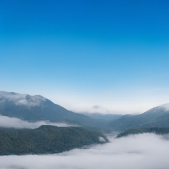
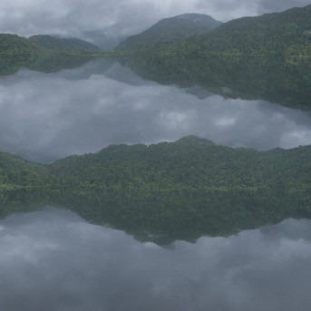
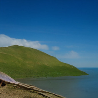
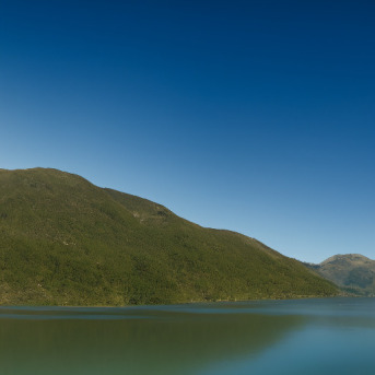
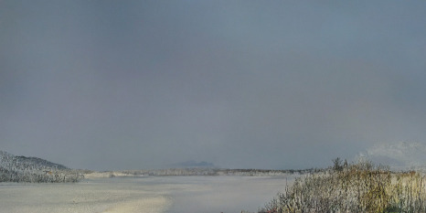
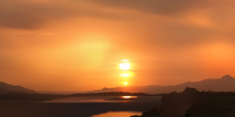
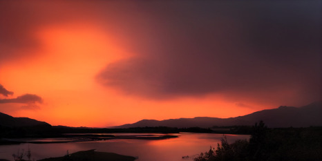
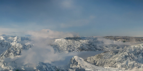
마지막으로, 우리는 landscapes 모델(Fig.12, 23, 24및25), class-conditional ImageNet 모델(Fig.26 - 27) 및 CelebA-HQ, FFHQ와 LSUN 데이터셋에 대한 unconditional 모델(Fig.28 - 31). Sec.의 inpainting 모델과 유사하게4.5우리는 또한 Sec.의 semantic landscapes 모델을 fine-tune했다4.3.2직접 다음에서${512}^2$이미지로 하고 정성적 결과를 Fig.에 묘사한다12및 Fig.23. 비교적 작은 데이터셋에서 훈련된 우리의 이러한 모델들에 대해, 우리는 추가로 VGG에서의 nearest neighbors를 보여준다[79]우리 모델들의 샘플에 대한 feature space를 Fig.에서32 - 34.

Flickr-Landscapes에서의 Semantic Synthesis[23] (${512}^2$finetuning)

Figure 23: Sec.에서와 같은 semantic landscapes 모델의 convolutional samples4.3.2, 다음에서 finetune됨${512}^2$이미지.

Figure 24: A LDM다음에서 훈련된${256}^2$해상도는 landscape 이미지의 semantic synthesis와 같은 spatially conditioned tasks에 대해 더 큰 해상도로 일반화할 수 있다. Sec. 참조4.3.2.

Flickr-Landscapes에서의 Semantic Synthesis[23]

Figure 25: semantic map이 conditioning으로 제공될 때, 우리의LDMs훈련 중 본 것보다 상당히 더 큰 해상도로 일반화한다. 이 모델은 크기의 입력에서 훈련되었지만${256}^2$여기에 보이는 것과 같은 고해상도 샘플을 생성하는 데 사용될 수 있으며, 이들은 해상도가 다음이다$1024\times 384$.

ImageNet 데이터셋에서의 무작위 class conditional samples

Figure 26: 다음으로부터의 무작위 샘플LDM-4ImageNet 데이터셋에서 훈련됨. classifier-free guidance로 샘플링됨[32]scale$s=5.0$및 다음과 함께 200 DDIM steps$\eta =1.0$.

ImageNet 데이터셋에서의 무작위 class conditional samples

Figure 27: 다음으로부터의 무작위 샘플LDM-4ImageNet 데이터셋에서 훈련됨. classifier-free guidance로 샘플링됨[32]scale$s=3.0$및 다음과 함께 200 DDIM steps$\eta =1.0$.

CelebA-HQ 데이터셋에서의 무작위 샘플

Figure 28: 우리의 최고 성능 모델의 무작위 샘플LDM-4CelebA-HQ 데이터셋에서. 500 DDIM steps 및 다음과 함께 샘플링됨$\eta =0$(FID = 5.15).

FFHQ 데이터셋에서의 무작위 샘플

Figure 29: 우리의 최고 성능 모델의 무작위 샘플LDM-4FFHQ 데이터셋에서. 200 DDIM steps 및 다음과 함께 샘플링됨$\eta =1$(FID = 4.98).

LSUN-Churches 데이터셋에서의 무작위 샘플

Figure 30: 우리의 최고 성능 모델의 무작위 샘플LDM-8LSUN-Churches 데이터셋에서. 200 DDIM steps 및 다음과 함께 샘플링됨$\eta =0$(FID = 4.48).

LSUN-Bedrooms 데이터셋에서의 무작위 샘플

Figure 31: 우리의 최고 성능 모델의 무작위 샘플LDM-4LSUN-Bedrooms 데이터셋에서. 200 DDIM steps 및 다음과 함께 샘플링됨$\eta =1$(FID = 2.95).

CelebA-HQ 데이터셋에서의 Nearest Neighbors

Figure 32: VGG-16의 feature space에서 계산된 우리의 최고 CelebA-HQ 모델의 nearest neighbors[79]. 가장 왼쪽 샘플은 우리 모델에서 온 것이다. 각 행의 나머지 샘플들은 그것의 10 nearest neighbors이다.

FFHQ 데이터셋에서의 Nearest Neighbors

Figure 33: VGG-16의 feature space에서 계산된 우리의 최고 FFHQ 모델의 nearest neighbors[79]. 가장 왼쪽 샘플은 우리 모델에서 온 것이다. 각 행의 나머지 샘플들은 그것의 10 nearest neighbors이다.

LSUN-Churches 데이터셋에서의 Nearest Neighbors

Figure 34: VGG-16의 feature space에서 계산된 우리의 최고 LSUN-Churches 모델의 nearest neighbors[79]. 가장 왼쪽 샘플은 우리 모델에서 온 것이다. 각 행의 나머지 샘플들은 그것의 10 nearest neighbors이다.

References

- [1] Eirikur Agustsson and Radu Timofte. 단일 이미지 super-resolution에 대한 NTIRE 2017 challenge: Dataset and study. In2017 IEEE Conference on Computer Vision and Pattern Recognition Workshops, CVPR Workshops 2017, Honolulu, HI, USA, July 21-26, 2017, pages 1122–1131. IEEE Computer Society, 2017.
- [2] Martin Arjovsky, Soumith Chintala, and Léon Bottou. Wasserstein gan, 2017.
- [3] Andrew Brock, Jeff Donahue, and Karen Simonyan. 고충실도 자연 이미지 합성을 위한 대규모 GAN training. InInt. Conf. Learn. Represent., 2019.
- [4] Holger Caesar, Jasper R. R. Uijlings, and Vittorio Ferrari. Coco-stuff: 맥락 속의 thing 및 stuff classes. In2018 IEEE Conference on Computer Vision and Pattern Recognition, CVPR 2018, Salt Lake City, UT, USA, June 18-22, 2018, pages 1209–1218. Computer Vision Foundation / IEEE Computer Society, 2018.
- [5] Nicholas Carlini, Florian Tramer, Eric Wallace, Matthew Jagielski, Ariel Herbert-Voss, Katherine Lee, Adam Roberts, Tom Brown, Dawn Song, Ulfar Erlingsson, et al. large language models로부터 training data 추출. In30th USENIX Security Symposium (USENIX Security 21), pages 2633–2650, 2021.
- [6] Mark Chen, Alec Radford, Rewon Child, Jeffrey Wu, Heewoo Jun, David Luan, and Ilya Sutskever. pixels로부터의 generative pretraining. InICML, volume 119 ofProceedings of Machine Learning Research, pages 1691–1703. PMLR, 2020.
- [7] Nanxin Chen, Yu Zhang, Heiga Zen, Ron J. Weiss, Mohammad Norouzi, and William Chan. Wavegrad: waveform generation을 위한 gradients 추정. InICLR. OpenReview.net, 2021.
- [8] Lu Chi, Borui Jiang, and Yadong Mu. Fast fourier convolution. InNeurIPS, 2020.
- [9] Rewon Child. 매우 깊은 vaes는 autoregressive models를 일반화하고 images에서 그것들을 능가할 수 있다. CoRR, abs/2011.10650, 2020.
- [10] Rewon Child, Scott Gray, Alec Radford, and Ilya Sutskever. sparse transformers로 긴 sequences 생성. CoRR, abs/1904.10509, 2019.
- [11] Bin Dai and David P. Wipf. VAE models 진단 및 향상. InICLR (Poster). OpenReview.net, 2019.
- [12] Jia Deng, Wei Dong, Richard Socher, Li-Jia Li, Kai Li, and Fei-Fei Li. Imagenet: 대규모 계층적 이미지 데이터베이스. InCVPR, pages 248–255. IEEE Computer Society, 2009.
- [13] Emily Denton. generative ai의 윤리적 고려사항. AI for Content Creation Workshop, CVPR, 2021.
- [14] Jacob Devlin, Ming-Wei Chang, Kenton Lee, and Kristina Toutanova. BERT: 언어 이해를 위한 deep bidirectional transformers의 사전 학습. CoRR, abs/1810.04805, 2018.
- [15] Prafulla Dhariwal and Alex Nichol. Diffusion models는 이미지 합성에서 gans를 능가한다. CoRR, abs/2105.05233, 2021.
- [16] Sander Dieleman. typicality에 대한 단상, 2020.
- [17] Ming Ding, Zhuoyi Yang, Wenyi Hong, Wendi Zheng, Chang Zhou, Da Yin, Junyang Lin, Xu Zou, Zhou Shao, Hongxia Yang, and Jie Tang. Cogview: transformers를 통한 text-to-image 생성 숙달. CoRR, abs/2105.13290, 2021.
- [18] Laurent Dinh, David Krueger, and Yoshua Bengio. Nice: Non-linear independent components estimation, 2015.
- [19] Laurent Dinh, Jascha Sohl-Dickstein, and Samy Bengio. real NVP를 사용한 밀도 추정. 에서5th International Conference on Learning Representations, ICLR 2017, Toulon, France, April 24-26, 2017, Conference Track Proceedings. OpenReview.net, 2017.
- [20] Alexey Dosovitskiy and Thomas Brox. deep networks에 기반한 perceptual similarity metrics로 이미지 생성. Daniel D. Lee, Masashi Sugiyama, Ulrike von Luxburg, Isabelle Guyon, and Roman Garnett, 편집자, 에서Adv. Neural Inform. Process. Syst., pages 658–666, 2016.
- [21] Patrick Esser, Robin Rombach, Andreas Blattmann, and Björn Ommer. Imagebart: autoregressive 이미지 합성을 위한 multinomial diffusion을 사용한 bidirectional context. CoRR, abs/2108.08827, 2021.
- [22] Patrick Esser, Robin Rombach, and Björn Ommer. generative models에서의 data biases에 관한 노트. arXiv preprint arXiv:2012.02516, 2020.
- [23] Patrick Esser, Robin Rombach, and Björn Ommer. 고해상도 이미지 합성을 위한 transformers 길들이기. CoRR, abs/2012.09841, 2020.
- [24] Mary Anne Franks and Ari Ezra Waldman. Sex, lies, and videotape: Deep fakes와 free speech delusions. Md. L. Rev., 78:892, 2018.
- [25] Kevin Frans, Lisa B. Soros, and Olaf Witkowski. Clipdraw: language-image encoders를 통한 text-to-drawing 합성 탐구. ArXiv, abs/2106.14843, 2021.
- [26] Oran Gafni, Adam Polyak, Oron Ashual, Shelly Sheynin, Devi Parikh, and Yaniv Taigman. Make-a-scene: human priors를 사용한 scene-based text-to-image 생성. CoRR, abs/2203.13131, 2022.
- [27] Ian J. Goodfellow, Jean Pouget-Abadie, Mehdi Mirza, Bing Xu, David Warde-Farley, Sherjil Ozair, Aaron C. Courville, and Yoshua Bengio. Generative adversarial networks. CoRR, 2014.
- [28] Ishaan Gulrajani, Faruk Ahmed, Martin Arjovsky, Vincent Dumoulin, and Aaron Courville. wasserstein gans의 개선된 훈련, 2017.
- [29] Martin Heusel, Hubert Ramsauer, Thomas Unterthiner, Bernhard Nessler, and Sepp Hochreiter. two time-scale update rule로 훈련된 Gans는 local nash equilibrium으로 수렴한다. 에서Adv. Neural Inform. Process. Syst., pages 6626–6637, 2017.
- [30] Jonathan Ho, Ajay Jain, and Pieter Abbeel. Denoising diffusion probabilistic models. 에서NeurIPS, 2020.
- [31] Jonathan Ho, Chitwan Saharia, William Chan, David J. Fleet, Mohammad Norouzi, and Tim Salimans. 고충실도 이미지 생성을 위한 Cascaded diffusion models. CoRR, abs/2106.15282, 2021.
- [32] Jonathan Ho and Tim Salimans. Classifier-free diffusion guidance. 에서NeurIPS 2021 Workshop on Deep Generative Models and Downstream Applications, 2021.
- [33] Phillip Isola, Jun-Yan Zhu, Tinghui Zhou, and Alexei A. Efros. conditional adversarial networks를 사용한 Image-to-image translation. 에서CVPR, pages 5967–5976. IEEE Computer Society, 2017.
- [34] Phillip Isola, Jun-Yan Zhu, Tinghui Zhou, and Alexei A. Efros. conditional adversarial networks를 사용한 Image-to-image translation. 2017 IEEE Conference on Computer Vision and Pattern Recognition (CVPR), pages 5967–5976, 2017.
- [35] Andrew Jaegle, Sebastian Borgeaud, Jean-Baptiste Alayrac, Carl Doersch, Catalin Ionescu, David Ding, Skanda Koppula, Daniel Zoran, Andrew Brock, Evan Shelhamer, Olivier J. Hénaff, Matthew M. Botvinick, Andrew Zisserman, Oriol Vinyals, and João Carreira. Perceiver IO: 구조화된 입력을 위한 일반 아키텍처&출력. CoRR, abs/2107.14795, 2021.
- [36] Andrew Jaegle, Felix Gimeno, Andy Brock, Oriol Vinyals, Andrew Zisserman, and João Carreira. Perceiver: iterative attention을 사용한 일반 지각. Marina Meila and Tong Zhang, 편집자, 에서Proceedings of the 38th International Conference on Machine Learning, ICML 2021, 18-24 July 2021, Virtual Event, volume 139 ofProceedings of Machine Learning Research, pages 4651–4664. PMLR, 2021.
- [37] Manuel Jahn, Robin Rombach, and Björn Ommer. transformers를 사용한 고해상도 복잡 장면 합성. CoRR, abs/2105.06458, 2021.
- [38] Niharika Jain, Alberto Olmo, Sailik Sengupta, Lydia Manikonda, and Subbarao Kambhampati. Imperfect imaganation: GANs가 얼굴 데이터 증강과 snapchat selfie lenses에서 편향을 악화시키는 것의 함의. arXiv preprint arXiv:2001.09528, 2020.
- [39] Tero Karras, Timo Aila, Samuli Laine, and Jaakko Lehtinen. 향상된 품질, 안정성, 변형을 위한 gans의 progressive growing. CoRR, abs/1710.10196, 2017.
- [40] Tero Karras, Samuli Laine, and Timo Aila. generative adversarial networks를 위한 style-based generator architecture. 에서IEEE Conf. Comput. Vis. Pattern Recog., pages 4401–4410, 2019.
- [41] T. Karras, S. Laine, and T. Aila. generative adversarial networks를 위한 style-based generator architecture. 에서2019 IEEE/CVF Conference on Computer Vision and Pattern Recognition (CVPR), 2019.
- [42] Tero Karras, Samuli Laine, Miika Aittala, Janne Hellsten, Jaakko Lehtinen, and Timo Aila. stylegan의 이미지 품질 분석 및 개선. CoRR, abs/1912.04958, 2019.
- [43] Dongjun Kim, Seungjae Shin, Kyungwoo Song, Wanmo Kang, and Il-Chul Moon. 무한한 data score를 위한 Score matching model. CoRR, abs/2106.05527, 2021.
- [44] Durk P Kingma and Prafulla Dhariwal. Glow: invertible 1x1 convolutions를 사용한 generative flow. S. Bengio, H. Wallach, H. Larochelle, K. Grauman, N. Cesa-Bianchi, and R. Garnett, 편집자, 에서Advances in Neural Information Processing Systems, 2018.
- [45] Diederik P. Kingma, Tim Salimans, Ben Poole, and Jonathan Ho. Variational diffusion models. CoRR, abs/2107.00630, 2021.
- [46] Diederik P. Kingma and Max Welling. Auto-Encoding Variational Bayes. 에서2nd International Conference on Learning Representations, ICLR, 2014.
- [47] Zhifeng Kong and Wei Ping. diffusion probabilistic models의 빠른 샘플링에 관하여. CoRR, abs/2106.00132, 2021.
- [48] Zhifeng Kong, Wei Ping, Jiaji Huang, Kexin Zhao, and Bryan Catanzaro. Diffwave: 오디오 합성을 위한 다목적 diffusion model. 에서ICLR. OpenReview.net, 2021.
- [49] Alina Kuznetsova, Hassan Rom, Neil Alldrin, Jasper R. R. Uijlings, Ivan Krasin, Jordi Pont-Tuset, Shahab Kamali, Stefan Popov, Matteo Malloci, Tom Duerig, and Vittorio Ferrari. The open images dataset V4: 대규모의 통합 이미지 분류, 객체 감지, 시각적 관계 감지. CoRR, abs/1811.00982, 2018.
- [50] Tuomas Kynkäänniemi, Tero Karras, Samuli Laine, Jaakko Lehtinen, and Timo Aila. generative models 평가를 위한 개선된 precision and recall metric. CoRR, abs/1904.06991, 2019.
- [51] Tsung-Yi Lin, Michael Maire, Serge J. Belongie, Lubomir D. Bourdev, Ross B. Girshick, James Hays, Pietro Perona, Deva Ramanan, Piotr Dollár, and C. Lawrence Zitnick. Microsoft COCO: context 속 common objects. CoRR, abs/1405.0312, 2014.
- [52] Yuqing Ma, Xianglong Liu, Shihao Bai, Le-Yi Wang, Aishan Liu, Dacheng Tao, and Edwin Hancock. 큰 결손 영역을 위한 region-wise generative adversarial imageinpainting. ArXiv, abs/1909.12507, 2019.
- [53] Chenlin Meng, Yang Song, Jiaming Song, Jiajun Wu, Jun-Yan Zhu, and Stefano Ermon. Sdedit: stochastic differential equations를 사용한 이미지 합성 및 편집. CoRR, abs/2108.01073, 2021.
- [54] Lars M. Mescheder. GAN training의 convergence properties에 관하여. CoRR, abs/1801.04406, 2018.
- [55] Luke Metz, Ben Poole, David Pfau, and Jascha Sohl-Dickstein. Unrolled generative adversarial networks. 에서5th International Conference on Learning Representations, ICLR 2017, Toulon, France, April 24-26, 2017, Conference Track Proceedings. OpenReview.net, 2017.
- [56] Mehdi Mirza and Simon Osindero. Conditional generative adversarial nets. CoRR, abs/1411.1784, 2014.
- [57] Gautam Mittal, Jesse H. Engel, Curtis Hawthorne, and Ian Simon. diffusion models를 사용한 symbolic music generation. CoRR, abs/2103.16091, 2021.
- [58] Kamyar Nazeri, Eric Ng, Tony Joseph, Faisal Z. Qureshi, and Mehran Ebrahimi. Edgeconnect: adversarial edge learning을 사용한 generative image inpainting. ArXiv, abs/1901.00212, 2019.
- [59] Alex Nichol, Prafulla Dhariwal, Aditya Ramesh, Pranav Shyam, Pamela Mishkin, Bob McGrew, Ilya Sutskever, and Mark Chen. GLIDE: text-guided diffusion models를 사용한 photorealistic 이미지 생성 및 편집을 향하여. CoRR, abs/2112.10741, 2021.
- [60] Anton Obukhov, Maximilian Seitzer, Po-Wei Wu, Semen Zhydenko, Jonathan Kyl, and Elvis Yu-Jing Lin. pytorch에서 generative models를 위한 high-fidelity performance metrics, 2020. Version: 0.3.0, DOI: 10.5281/zenodo.4957738.
- [61] Taesung Park, Ming-Yu Liu, Ting-Chun Wang, and Jun-Yan Zhu. spatially-adaptive normalization을 사용한 semantic image synthesis. 에서Proceedings of the IEEE Conference on Computer Vision and Pattern Recognition, 2019.
- [62] Taesung Park, Ming-Yu Liu, Ting-Chun Wang, and Jun-Yan Zhu. spatially-adaptive normalization을 사용한 semantic image synthesis. 에서Proceedings of the IEEE/CVF Conference on Computer Vision and Pattern Recognition (CVPR), June 2019.
- [63] Gaurav Parmar, Dacheng Li, Kwonjoon Lee, and Zhuowen Tu. Dual contradistinctive generative autoencoder. InIEEE Conference on Computer Vision and Pattern Recognition, CVPR 2021, 가상, 2021년 6월 19-25일, pages 823–832. Computer Vision Foundation / IEEE, 2021.
- [64] Gaurav Parmar, Richard Zhang, and Jun-Yan Zhu. 버그가 있는 리사이징 라이브러리와 fid 계산에서의 놀라운 미묘함에 관하여. arXiv preprint arXiv:2104.11222, 2021.
- [65] David A. Patterson, Joseph Gonzalez, Quoc V. Le, Chen Liang, Lluis-Miquel Munguia, Daniel Rothchild, David R. So, Maud Texier, and Jeff Dean. 탄소 배출과 대규모 신경망 훈련. CoRR, abs/2104.10350, 2021.
- [66] Aditya Ramesh, Mikhail Pavlov, Gabriel Goh, Scott Gray, Chelsea Voss, Alec Radford, Mark Chen, and Ilya Sutskever. Zero-shot text-to-image generation. CoRR, abs/2102.12092, 2021.
- [67] Ali Razavi, Aäron van den Oord, and Oriol Vinyals. VQ-VAE-2로 다양한 고충실도 이미지를 생성하기. InNeurIPS, pages 14837–14847, 2019.
- [68] Scott E. Reed, Zeynep Akata, Xinchen Yan, Lajanugen Logeswaran, Bernt Schiele, and Honglak Lee. 생성적 적대적 텍스트에서 이미지 합성. InICML, 2016.
- [69] Danilo Jimenez Rezende, Shakir Mohamed, and Daan Wierstra. 심층 생성 모델에서의 확률적 역전파와 근사 추론. InProceedings of the 31st International Conference on International Conference on Machine Learning, ICML, 2014.
- [70] Robin Rombach, Patrick Esser, and Björn Ommer. 조건부 가역 신경망을 이용한 네트워크-대-네트워크 변환. InNeurIPS, 2020.
- [71] Olaf Ronneberger, Philipp Fischer, and Thomas Brox. U-net: 생의학 이미지 분할을 위한 합성곱 네트워크. InMICCAI (3), volume 9351 ofLecture Notes in Computer Science, pages 234–241. Springer, 2015.
- [72] Chitwan Saharia, Jonathan Ho, William Chan, Tim Salimans, David J. Fleet, and Mohammad Norouzi. 반복적 정제를 통한 이미지 초해상도. CoRR, abs/2104.07636, 2021.
- [73] Tim Salimans, Andrej Karpathy, Xi Chen, and Diederik P. Kingma. Pixelcnn++: 이산화된 로지스틱 혼합 우도와 기타 수정으로 pixelcnn 개선하기. CoRR, abs/1701.05517, 2017.
- [74] Dave Salvator. NVIDIA Developer Blog. https://developer.nvidia.com/blog/getting-immediate-speedups-with-a100-tf32, 2020.
- [75] Robin San-Roman, Eliya Nachmani, and Lior Wolf. 생성적 diffusion 모델을 위한 노이즈 추정. CoRR, abs/2104.02600, 2021.
- [76] Axel Sauer, Kashyap Chitta, Jens Müller, and Andreas Geiger. Projected gans는 더 빠르게 수렴한다. CoRR, abs/2111.01007, 2021.
- [77] Edgar Schönfeld, Bernt Schiele, and Anna Khoreva. 생성적 적대 신경망을 위한 u-net 기반 판별기. In2020 IEEE/CVF Conference on Computer Vision and Pattern Recognition, CVPR 2020, Seattle, WA, USA, 2020년 6월 13-19일, pages 8204–8213. Computer Vision Foundation / IEEE, 2020.
- [78] Christoph Schuhmann, Richard Vencu, Romain Beaumont, Robert Kaczmarczyk, Clayton Mullis, Aarush Katta, Theo Coombes, Jenia Jitsev, and Aran Komatsuzaki. Laion-400m: clip으로 필터링된 4억 개 이미지-텍스트 쌍의 공개 데이터셋, 2021.
- [79] Karen Simonyan and Andrew Zisserman. 대규모 이미지 인식을 위한 매우 깊은 합성곱 네트워크. In Yoshua Bengio and Yann LeCun, editors,Int. Conf. Learn. Represent., 2015.
- [80] Abhishek Sinha, Jiaming Song, Chenlin Meng, and Stefano Ermon. D2C: few-shot 조건부 생성을 위한 diffusion-denoising 모델. CoRR, abs/2106.06819, 2021.
- [81] Charlie Snell. Alien Dreams: 떠오르는 예술 장면. https://ml.berkeley.edu/blog/posts/clip-art/, 2021. [Online; 2021년 11월에 접근됨].
- [82] Jascha Sohl-Dickstein, Eric A. Weiss, Niru Maheswaranathan, and Surya Ganguli. 비평형 열역학을 이용한 심층 비지도 학습. CoRR, abs/1503.03585, 2015.
- [83] Kihyuk Sohn, Honglak Lee, and Xinchen Yan. 심층 조건부 생성 모델을 이용한 구조화된 출력 표현 학습. In C. Cortes, N. Lawrence, D. Lee, M. Sugiyama, and R. Garnett, editors,Advances in Neural Information Processing Systems, volume 28. Curran Associates, Inc., 2015.
- [84] Jiaming Song, Chenlin Meng, and Stefano Ermon. Denoising diffusion implicit models. InICLR. OpenReview.net, 2021.
- [85] Yang Song, Jascha Sohl-Dickstein, Diederik P. Kingma, Abhishek Kumar, Stefano Ermon, and Ben Poole. 확률 미분 방정식을 통한 score-based 생성 모델링. CoRR, abs/2011.13456, 2020.
- [86] Emma Strubell, Ananya Ganesh, and Andrew McCallum. 현대 딥러닝 연구를 위한 에너지 및 정책 고려사항. InThe Thirty-Fourth AAAI Conference on Artificial Intelligence, AAAI 2020, The Thirty-Second Innovative Applications of Artificial Intelligence Conference, IAAI 2020, The Tenth AAAI Symposium on Educational Advances in Artificial Intelligence, EAAI 2020, New York, NY, USA, 2020년 2월 7-12일, pages 13693–13696. AAAI Press, 2020.
- [87] Wei Sun and Tianfu Wu. 제어 가능한 이미지 합성을 위한 레이아웃 및 스타일 재구성 가능한 gans 학습. CoRR, abs/2003.11571, 2020.
- [88] Roman Suvorov, Elizaveta Logacheva, Anton Mashikhin, Anastasia Remizova, Arsenii Ashukha, Aleksei Silvestrov, Naejin Kong, Harshith Goka, Kiwoong Park, and Victor S. Lempitsky. fourier convolutions를 이용한 해상도-강건 대형 마스크 인페인팅. ArXiv, abs/2109.07161, 2021.
- [89] Tristan Sylvain, Pengchuan Zhang, Yoshua Bengio, R. Devon Hjelm, and Shikhar Sharma. 레이아웃으로부터의 객체 중심 이미지 생성. InThirty-Fifth AAAI Conference on Artificial Intelligence, AAAI 2021, Thirty-Third Conference on Innovative Applications of Artificial Intelligence, IAAI 2021, The Eleventh Symposium on Educational Advances in Artificial Intelligence, EAAI 2021, Virtual Event, 2021년 2월 2-9일, pages 2647–2655. AAAI Press, 2021.
- [90] Patrick Tinsley, Adam Czajka, and Patrick Flynn. 이 얼굴은 존재하지 않는다… 하지만 당신의 것일 수도 있다! 생성 모델에서의 정체성 누출. InProceedings of the IEEE/CVF Winter Conference on Applications of Computer Vision, pages 1320–1328, 2021.
- [91] Antonio Torralba and Alexei A Efros. 데이터셋 편향에 대한 편향 없는 시각. InCVPR 2011, pages 1521–1528. IEEE, 2011.
- [92] Arash Vahdat and Jan Kautz. NVAE: 심층 계층적 변분 오토인코더. InNeurIPS, 2020.
- [93] Arash Vahdat, Karsten Kreis, and Jan Kautz. 잠재 공간에서의 score-based 생성 모델링. CoRR, abs/2106.05931, 2021.
- [94] Aaron van den Oord, Nal Kalchbrenner, Lasse Espeholt, koray kavukcuoglu, Oriol Vinyals, and Alex Graves. pixelcnn 디코더를 이용한 조건부 이미지 생성. InAdvances in Neural Information Processing Systems, 2016.
- [95] Aäron van den Oord, Nal Kalchbrenner, and Koray Kavukcuoglu. Pixel recurrent neural networks. CoRR, abs/1601.06759, 2016.
- [96] Aäron van den Oord, Oriol Vinyals, and Koray Kavukcuoglu. 신경 이산 표현 학습. InNIPS, pages 6306–6315, 2017.
- [97] Ashish Vaswani, Noam Shazeer, Niki Parmar, Jakob Uszkoreit, Llion Jones, Aidan N. Gomez, Lukasz Kaiser, and Illia Polosukhin. Attention is all you need. InNIPS, pages 5998–6008, 2017.
- [98] Rivers Have Wings. 자기회귀 모델을 위한 Classifier-free guidance에 관한 트윗. https://twitter.com/RiversHaveWings/status/1478093658716966912, 2022.
- [99] Thomas Wolf, Lysandre Debut, Victor Sanh, Julien Chaumond, Clement Delangue, Anthony Moi, Pierric Cistac, Tim Rault, Rémi Louf, Morgan Funtowicz, and Jamie Brew. Huggingface의 transformers: 최첨단 자연어 처리. CoRR, abs/1910.03771, 2019.
- [100] Zhisheng Xiao, Karsten Kreis, Jan Kautz, and Arash Vahdat. VAEBM: 변분 오토인코더와 에너지 기반 모델 사이의 공생. In9th International Conference on Learning Representations, ICLR 2021, Virtual Event, Austria, 2021년 5월 3-7일. OpenReview.net, 2021.
- [101] Wilson Yan, Yunzhi Zhang, Pieter Abbeel, and Aravind Srinivas. Videogpt: VQ-VAE와 transformers를 이용한 비디오 생성. CoRR, abs/2104.10157, 2021.
- [102] Fisher Yu, Yinda Zhang, Shuran Song, Ari Seff, and Jianxiong Xiao. LSUN: 인간을 루프 안에 둔 딥러닝을 이용한 대규모 이미지 데이터셋의 구축. CoRR, abs/1506.03365, 2015.
- [103] Jiahui Yu, Xin Li, Jing Yu Koh, Han Zhang, Ruoming Pang, James Qin, Alexander Ku, Yuanzhong Xu, Jason Baldridge, and Yonghui Wu. 개선된 vqgan을 이용한 벡터 양자화 이미지 모델링, 2021.
- [104] Jiahui Yu, Zhe L. Lin, Jimei Yang, Xiaohui Shen, Xin Lu, and Thomas S. Huang. gated convolution을 이용한 자유 형식 이미지 인페인팅. 2019 IEEE/CVF International Conference on Computer Vision (ICCV), pages 4470–4479, 2019.
- [105] K. Zhang, Jingyun Liang, Luc Van Gool, and Radu Timofte. 심층 블라인드 이미지 초해상도를 위한 실용적인 열화 모델 설계. ArXiv, abs/2103.14006, 2021.
- [106] Richard Zhang, Phillip Isola, Alexei A. Efros, Eli Shechtman, and Oliver Wang. 지각적 metric으로서 심층 특징의 불합리한 효과성. InProceedings of the IEEE Conference on Computer Vision and Pattern Recognition (CVPR), 2018년 6월.
- [107] Shengyu Zhao, Jianwei Cui, Yilun Sheng, Yue Dong, Xiao Liang, Eric I-Chao Chang, and Yan Xu. 공동 변조된 생성적 적대 신경망을 통한 대규모 이미지 완성. ArXiv, abs/2103.10428, 2021.
- [108] Bolei Zhou, Àgata Lapedriza, Aditya Khosla, Aude Oliva, and Antonio Torralba. Places: 장면 인식을 위한 1,000만 이미지 데이터베이스. IEEE Transactions on Pattern Analysis and Machine Intelligence, 40:1452–1464, 2018.
- [109] Yufan Zhou, Ruiyi Zhang, Changyou Chen, Chunyuan Li, Chris Tensmeyer, Tong Yu, Jiuxiang Gu, Jinhui Xu, and Tong Sun. LAFITE: text-to-image generation을 위한 언어 없는 훈련을 향하여. CoRR, abs/2111.13792, 2021.